GLM for Correlated Data

So far the models we've covered assume independence between observations collected on separate individuals. When observation are correlated models that incorporate the existing correlation in the data should be employed. There are many approaches are proposed but here we focus on Generalized Estimating Equations (GEE) and Mixed Effects Generalized Linear Models.

Generalized Estimating Equations Methods

For classical generalized linear model we assume only one observation was collected per subject with a set of predictors.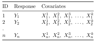

The most common type of correlated data is longitudinal, collected on the same subjects over time. For data with 3 time points: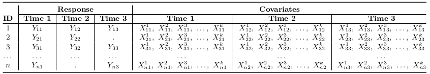

Other examples of correlated data are: Data collected from different locations on the same subject or collected on different subjects which are related.

In SAS the function to estimate GEE models is PROC GENMOD. For normal models it can be fit in other procedures, such as PROC MIXED. Using PROC GENMOD the data must be inputted in long form (multiple observations per subject):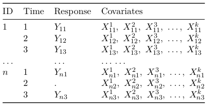

Now we could analyze the data by observing the counts out the outcome while ignoring the correlation between subjects, or simply observe the linear correlation between outcome and time, but in general ignoring the dependency of the observations will in general overestimate the standard errors of the time-dependent predictors since we haven't accounted for within-subject variability.

The influence of correlation on statistical inference can be observed by inspecting its influence on the sample size for a design that collects data repeatedly over time. In comparing 2 groups in terms of means on a measured outcome Y_ij where i is subjects and j is group, and in each group there are m subjects and within each group there are n repeated observations. Further assuming that Var(Y_ij) = σ² and that within each group Cor(Y_ij, Y_hj) = ρ where i != h. Then the sample size needed to detect a difference in means of outcome, d = μ₁ + μ₂ = E(Y_i1) - E(Y_i2) with power P = 1 - Q and type I error (α) is:

$$ m = {{2(z\alpha + zQ)^2\sigma(sigma^2(1 + (n - 1)\rho)} \over {nd^2}} = {{2(z\alpha + zQ)^2\sigma^2(1 + (n - 1)\rho)} \over {n\Delta^2}}$$

Where \(\Delta = d / \sigma \) is the mean difference in standard deviation units. From the formula, the higher the correlation (ρ) the larger the larger the m.

However, standard errors of the time-independent predictors (such as treatment) will be underestimated. The long form of the data makes it seem like there's 4 times as much data then there really is. In comparing 2 groups in terms of slopes (rate of change) on a measured outcome, the sample size needed to detect a difference in slopes of a predictor x_h and outcome d = β₁ - β₂ with power P = 1 - Q is:

$$ m = {{2(z\alpha + zQ)^2\sigma^2(1 - \rho)} \over {ns^2_xd^2}} $$

Where \( s^2_x = \sum_j {(x_j \bar x)^2} \over n \) is the subject variance of the covariate values x_j. From the above formula the higher the correlation the smaller the m.