Hierarchical Models
Previously we have assumed given covariates, the observations are independent. However, there are many situations where this does not hold. Bayesian Hierarchical models can be used to cluster observations, where each cluster might have its own cluster-specific parameters.
In Bayesian hierarchical models, we start by imposing a prior that is a function of different parameters. We'll introduce a new variable γ, which is called the hyper-prior; The prior of α depends on β, which depends on γ.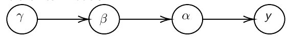
Hyper-parameters: Parameters of prior distribution
Hyper-Priors: Distribution of Hyper-parameters
A typical example of this in medical research is population of hospitals, providers within hospitals, and patients within providers. Any datasets with such a structure are called hierarchical. Hierarchical models are also called partial pooled or random effect models.
We are interested in making inference of specific units. In doing so observations may be collected over time on the same individuals, so repeated measures must be accounted for.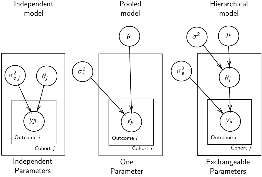
- Independent models have no randomly-varying effects
- Pooled models have a randomly-varying (subject-specific) effects of slope
- Hierarchical h ave randomly-varying (subject specific) effects of slope and intercept
Ranking Posterior Estimates
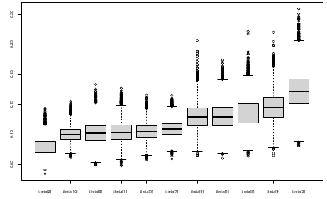
We can simply rank the outcome/results in a box plot such as the above, but this does not consider the uncertainty of the estimates.
We can derive the posterior distribution of each ranking by ranking the estimates at each iteration of the Gibbs Sampling and generate the posterior distributions of the ranks. Below the ranks are in parenthesis: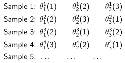
The posterior distribution of ranks gives us a measure of the uncertainty of the ordering.
Data Formatting
There are three main alternative approaches to account for the hierarchical structure of the data in coding, in order of popularity:
- Nested Indexes - Define an index of the same length of the data that specifies the cluster to which each unit belongs.
- Offset - Construct a vector of indexes that define the first and last element of each cluster. Needs two indexes
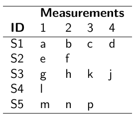
Tabular Format:
 Long Format:
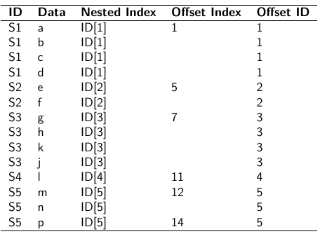
- Data padding - Structure data in array format and fill in empty cells with NA when clusters include different sample sizes

Model Implementation With Offset
### Begin by setting up the data and generating the offset
## Prepare outcome and covariate data
y <- na.omit(c(t(HB.data[, 6:8]))) # All outcome data
y0 <- HB.data[, 5] # Baseline data
t <- c(t(HB.data[, c(2, 3, 4)]))[-na.action(y)] # Times corresponding to non-missing outcome

## Fill in data for offset indexes one subject at a time, starting with the first subject
i <- 1
offset <- c(1, 1 + length(which(is.na(HB.data[1, 6:8]) == F)))

## Add a new offset for each subject until the end of data
while (offset[(i + 1)] < length(y) - 1) {
	i <- i + 1
	offset <- c(offset, offset[i] + length(which(is.na(HB.data[i,6:8]) == F))) # Calculate offsett for subject i
}
offset <- c(offset, (length(y) + 1)) # Concatenate to the set of offsets

model.1 <- "model {
	for (i in 1:N) {
		for(j in offset[i] : (offset[i+1]-1)){
			y[j] ~ dnorm(psi[j], tau.y)
			psi[j] <- alpha[i] + beta[i]*(t[j] - tbar)
				+ gamma*(y0[i] - y0bar)
		}
	alpha[i] ~ dnorm(mu.alpha, tau.alpha)
	beta[i] ~ dnorm(mu.beta, tau.beta)
	}
# priors
sigma.a <- 1/tau.alpha
sigma.b <- 1/tau.beta
sigma.y <- 1/tau.y
mu.alpha ~ dnorm(0, 0.0001)
mu.beta ~ dnorm(0, 0.0001)
gamma ~ dnorm(0, 0.0001)
tau.alpha ~dgamma(1,1)
tau.beta ~dgamma(1,1)
tau.y ~dgamma(1,1)
y0bar <- mean(y0[])
tbar <- mean(t[])
}"
i = subject
offset[i]: (offset[i + 1] -1) = observations corresponding to subject i
Comparing Hierarchical Models
Joint likelihood of data and parameters:![]()
There are three primary approaches used:
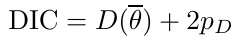
- Deviance Information Criterion (DIC)
Which is based on p(y | θ) - Akaike Information Criterion (AIC)
AIC = -2 log(y | φ̂) + 2pφ
where pφ is the number of hyper-parameters - Bayesian Information Criterion (BIC)
BIC = -2 log(y | φ̂) + log(n)*pφ

"Likelihood" is not well defined in a hierarchical model; It depends on the "focus" of the study if we want to use θ, φ, or the model structure without any unknown parameters. It is not a matter of which is correct but which is appropriate for our purpose.
Consider an example where our model predicts classes within schools in within a country:
- If we are interested in predicting future classes in those school then θ is the focus and deviance-based methods such as DIC are appropriate
- If we are interested in predicting results of future schools in a country then φ is the focus and marginal-likelihood methods such as AIC are appropriate; Relevant to education within the whole country.
- If we are interested in predicting results for a new country, then no parameters are in focus, the Bayes factors are appropriate to compare models; Relevant to general statements about education in the
- whole world or outside of the country being studied.