Bayesian Modeling - Logistic
Let Y be an indicator for presence of disease -> Y | p ~ Bin(p, 1)
Logistic regression models the log-ODDS (also called logit) of the mean outcome using a linear predictor.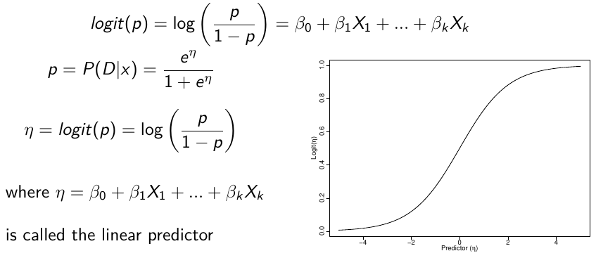
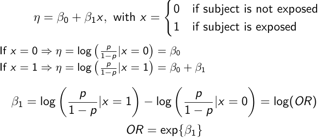
In a case-control study beta_0 is not interpretable. But the estimate of log(OR) can be interpreted correctly, given the symmetry of roles of disease/exposure
H0: OR = 1; Log(OR) = 0; No association
H1: OR != 1; Log(OR) != 0; Significant association
The Frequentist approach would be to simply fit a logistic regression in R using the function glm()
In Bayesian formulation we need to identify the parameters in our prior model, and the parameters we wish to estimate.
Ex. Below we model 2 parameters, beta_0 and beta_1, in a DAG model: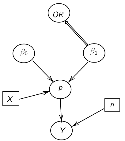
Because there's no constraint on the beta regression parameters, it is common to assume a normal distribution.
The magnitude of variance reflects the amount of uncertainty
In the below code:
- We loop to specify each observation
- Y.D[i] =
- 1 if subject i has the disease
- 0 if subject i does not have the disease
- X.E[i] =
- 1 if subject i has been exposed
- 0 if subject i has not been exposed
# Analysis with JAGS
library(rjags)

model.1 <- "model{
### data model
for(i in 1:N){
    Y.D[i] ~ dbin(p[i], 1)
    logit(p[i]) <- beta_0 + beta_1*X.E[i]
}
OR <- exp(beta_1)
pos.prob <- step(beta_1)
### prior
beta_1 ~ dnorm(0,0.0001)
beta_0 ~ dnorm(0,0.0001)
 0 i th subject unexposed
}"
# In R Data stored as a list
data.1 <- list(N = 331, X.E = X.E, Y.D = Y.D)
# Compile model (data is part of it!); `adapt` for 2,000 samples
model_odds <- jags.model(textConnection(model.1), data = data.1,
n.adapt = 2000)
update(model_odds, n.iter = 5000) # 5,000 burn-in samples
# Get 10,000 samples from the posterior distribution of OR, beta_0,beta_1
test_odds <- coda.samples(model_odds, c("OR", "beta_1", "beta_0"), n.iter = 10000)
plot(test_odds)
summary(test_odds)
In the output, we'll often look for the point estimate to be the posterior mean. However, when posterior density is skewed, posterior median is sometimes preferable.
Asymptotic Approximation
When the sample size is large enough, one can use an asymptotic approximation of the posterior distribution of the parameters.
When the sampling distribution is a member of the exponential family (Normal, Binomial, Poisson, or Gamma), then the posterior distribution of the parameters is (approximately) normally distribution: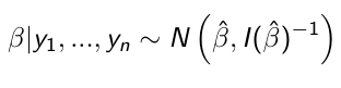 [1]
[1]
beta_hat is the ML (maximum likelihood) estimate of beta
I(beta_hat)^-1 is the Fisher Information matrix, evaluated in the ML estimate of beta
Based on the Maximum likelihood theory, asymptotically:![]() [2]
[2]
We don't need a prior in [1] because we have a lot of data. Results in [1] and [2] are close because the prior is weighted low because of the high sample size.