Bayesian Linear Regression
By now we know what a linear regression looks like. Let's consider a special case where number of parameters, p = 0: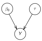
Assume Y is distributed as a normal distribution with mean β0:
Y|β0, τ ∼ N(β0, σ2 = 1/τ )
τ = 1 / σ2 , also called precision <- Be aware this will be used interchangeably with variance
The density function is: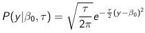
Mean and variance:
E(Y) = μ0; V(Y) = 1/τ0 + τ
The Posterior Distribution for β0 is calculated using Bayes' Theorem
When Mean and Variance are Unknown
We use a Normal prior distribution for the mean β0 ∼ N(μ0, τ0) and a Gamma prior distribution for the precision parameter: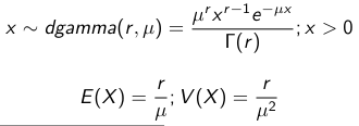
JAGS example:
model.1 <- "model {
	for (i in 1:N) {
		hbf[i] ~ dnorm(b.0,tau.t)
	}
	## prior on precision parameters
	tau.t ~ dgamma(1,1);
	### prior on mean given precision
	mu.0 <- 5
	tau.0 <- 0.44
	b.0 ~ dnorm(mu.0, tau.0);

    ### prediction
	hbf.new ~ dnorm(b.0,tau.t)
	pred <- step(hbf.new-20) # hbf >= 20
}"
Predictive Distributions
Given the Prior and Observed data we can compute the probability of a new observation will be greater or less than some integer threshold. The predictive distribution is a distribution of unobserved y~, that is: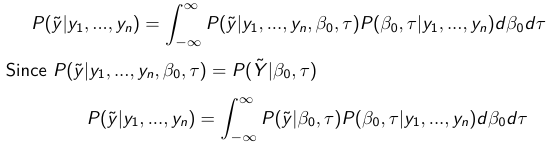
The two sources of variability in prediction are in the parameters V(β0, τ | y) and the variability in the new observation V(y | β0, τ)
- To simulate from predictive density, do repeatedly:
- Sample one sample β0*, τ* from posterior β0, τ | y
- Sample one y~ ~ N(β0*, 1/τ* )
- During the Gibbs sampling we generate samples values from the posterior distribution β0, τ | y
- So Generating y~ ~ N(β0, τ | y) will produce the correct predictive distribution samples. P(y~ > 20 | data) is the proportion of y~ > 20
Log Normal Distributions
Since in the example above the outcome distribution can only be positive we can use a Log-Normal distribution, a continuous distribution with support for values y > 0.
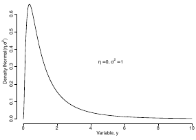
Y | η, σ2 ~ INormal(η, σ2) with density function: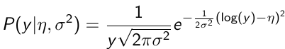
It also implies: Log( Y )~ Normal(η, σ2)
In JAGS we use: dlnorm(η, σ2)
"model {
for (i in 1:N) {
hbf[i] ~ dlnorm(lb.0,tau.t)
}
## prior on precision parameters
tau.t ~ dgamma(1,1);
### prior on mean
lb.0 ~ dnorm(1.6,1.6);
b.0 <- exp(lb.0)
### prediction
hbf.new ~ dlnorm(lb.0,tau.t)
pred <- step(hbf.new-20)
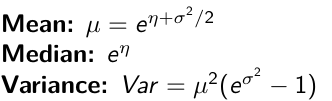
}"In the above example, we get the initial prior on β0 from previous data, where we derived median(b.0)=5 and V(b.0)=1/0.44=2.27
Then we take the log of the median to get η and transform the precision variable with: log(1 + V (b.0)/E (b.0)2 ), then take the inverse of that to get the variance.