Module 5: Multivariate Normal Distribution

A variable X follows a discrete probability distribution if the possible values of X are either:

• A finite set
• A countable infinite sequence

p_x(x_i) = P(X=x_i) is called the probability mass function (PMF)

• p_x(x_i)  >= 0 as it is a probability
  
• The sum of PMF for all values of X = 1

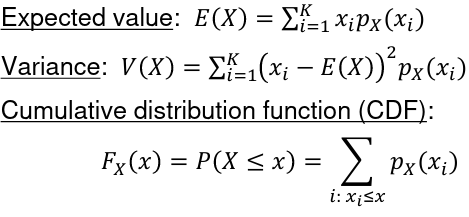
Recall that in a Discrete Probability Distribution :

In a Continuous Probability Distribution:

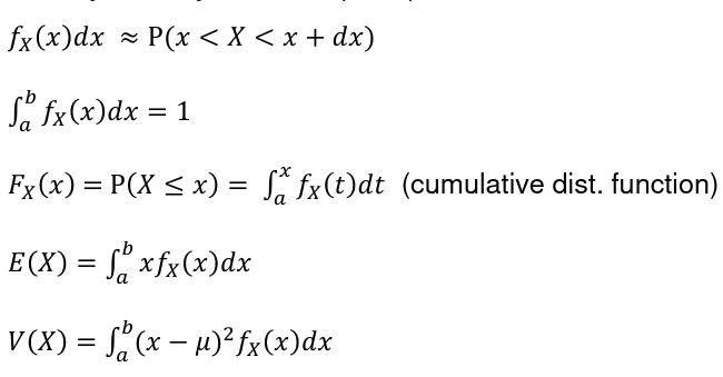
Because in a discrete set we are not concerned with the values in between our domain values.

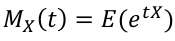
Moment Generating Function

Moments,Moments are expected values of X, such as E(X), V(X)E(X²) = E(V), E(X³), etc. This, can also be calculated using the Moment Generating Function (MGF):

The rth moment of X, E(X^r) can be obtained by differentiating M_x(t) r times with respect to t and setting t=0

• M_x(0) = 1
• M^I_x(0) = E(X)
• M^II_x(0) = E(X²) -> V(X) = M^II_x(0) - (MI_x(0))2
• In general, M_x^(r)(0) = E(X^r)

In short, the nth moment is the nth derivative of MGF.

Uniqueness: if X and Y are two random variables and M_x(t) = M_y(t) when |t| < h for some positive number h, then X and Y have the same distribution

Note: MGF does not exist for all distributions (E(e^tx) may be infinity)

Important Distributions

Normal Distribution

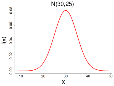
X ~ N(μ, σ²)        -infinity < μ < infinity , σ < 0

• PDF:

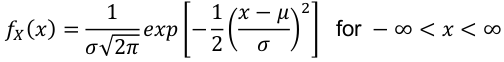
• E(X) = μ
• V(X) = σ²
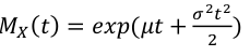
• MGF:

      

Binomial Distribution

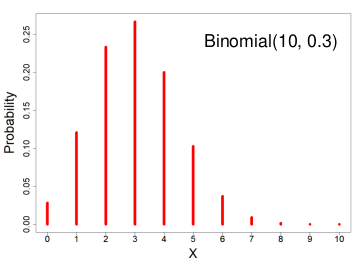
X ~ Binomial(n, p)      𝑝 ∈ [0, 1]

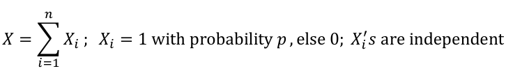
X = the number of successes in n trials when the probability of success in each trail is p.

We can think of X as the sum of n independent Bernoulli(p) random variables, with the same p for every X_i

• PMFPMF:
=

P(X

 = x) =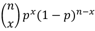      

• Expected value = E(X) = np
• Variance = V(X) = np(1-p)
• MGF = M_x(t) = (pe^t + (1-p))ⁿ
• Two discrete random variables are independent if: P(X = x & Y = y) = P(X = x)*P(Y=y)

Ex. A study which analyzed the prevalence of a disease in a population.

Poisson Distribution

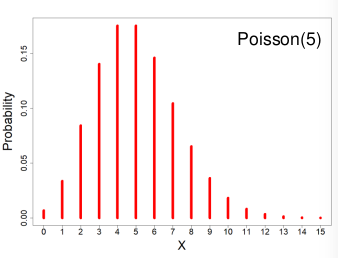
X ~ Poisson(λ)     λ > 0

X = The number of occurrences of an event of interest.

• PMFPMF:
=

       

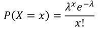
• Expected Values = E(X) = λ
• Variance = V(X) = λ
• MGF = M_x(t) = e^{λ(e^t - 1)}

Poisson as an approximation  of the Binomial Distribution

• If X ~ Binomial(n, p) and n -> infinity, p-> 0 such that np is a constant  =>  X ~ Poisson(np)
• This assumes each event is independent
• Often used analyzing rare diseases

Ex. Analyzing lung cancer in 1000 smokers and non-smokers. This is binomial but can be estimated as a Poisson distribution.

Geometric Distribution

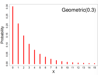
X ~ Geometric(p)      𝑝 ∈ (0, 1]

If Y₁, Y₂, Y₃ ... are a sequence of independent Bernoulli(p) random variables then the number of failures before the first success, X, follows a Geometric distribution.

• PMF = P(X = x) = p(1-p)^x
• Expected value = E(X) = (1-p)/p
• Variance = V(X) = (1-p)/p²
• MGF = M_x(t) = p / (1 - (1 - p)e^t)

Ex. We want to know the number of times to flip a coin before it lands on heads.

Hyper-Geometric Distribution

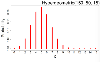
X ~ Hypergeometric(N, K, n)

Suppose a finite population of size N contains two mutually exclusive events: K success events and N-K failure events. If n events are randomly chosen without replacement X is the number of success events chosen.

• PMFPMF:
=

P(X

 = x) =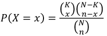      

• Expected value = E(X) = nk / N
• Variance = V(X) = ((nK) / N) * ((N-K) / N) * ((N - n) / (N - 1))

More

Ex. ImportantA Distributions

bag has 7 red beads and 13 white beads. If 5 are drawn without replacement what is the probability exactly 4 are red?

Uniform Distribution

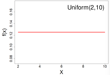
All outcomes are equally likely, they can be discrete or continuous.

X ~ Uniform(a, b)     a < b

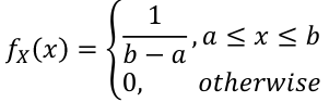
• PDFPDF:
=

       

• E(X) = (a + b)/2
• V(X) = (b - a)² / 12
• CDF = F(X) = (x - a) / (b -a), a<=x<=b
• MGFMGF:
=

       

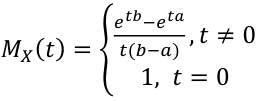
We use this distribution we use when we have no idea how the data is distributed.

Log-Normal Distribution

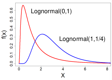
X ~ Lognormal(μ , σ²)    -infinity < μ  < infinity, σ > 0

• PDF:
  

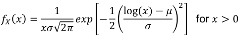
• E(X) = exp(μ + σ²/2)
• Median = e^μ
• V(X) = μ² * (e^{σ^2}-1)
  
• log(X) ~ N(μ, σ²)  - the log is normal
• These distributions are often skewed to the right

Ex. Amount of rainfall, production of milk by cows, or stock market fluctuation often follow logarithmic functions.

Gamma Distribution

X ~ Gamma(α, λ)    α > 0 , λ > 0

Exponential Distribution

A special subset of the Gamma Distribution (α = 1)

X ~ Exponential(λ)       λ  > 0

Chi-Square Distribution

Special case of the Gamma Distribution (α = k/2, λ = 1/2)

Properties of Gamma & Chi-Square Distribution

Distribution of the sum of independent Gamma random variables.

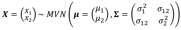
Bivariate Normal Distribution

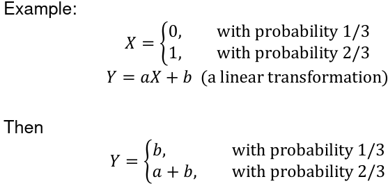
Function of a Discrete Random Variable

Suppose X is a discrete random variable and Y is a function of X.    Y = g(X)

The Y is also a random variable:   P(Y = y) = P(g(X) = y)

Function of a Continuous Random Variable

Using the same equation as above but assuming the variables are coninuous random variables:

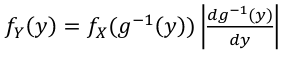
The PDF = 

The CDF =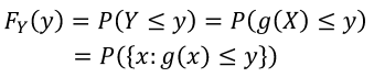 

If g is one-to-one (strictly increasing or decreasing) then g has an inverse g^-1, in the above case:

Covariance and Correlation

Correlation is defined as an indication as to how strong the relationship between the two variables is:

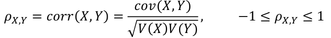
A positive correlation has σ > 0 and negative correlation has σ < 0

Covariance provides information about how the variables vary together:

    cov(X, Y) = R[(X - E(X))(Y - E(Y))]

This is also equivalent to:

    cov(X, Y) = E(XY) - E(X)*E(Y)

Thus if X and Y are independent:

    cov(X, Y) = corr(X, Y) = 0

Conditional Expectation of X given Y = y, denoted E(X | Y = y):

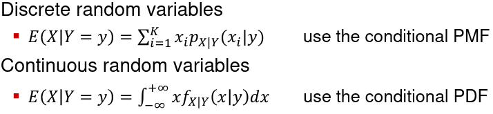
Conditional variance can be defined similarly (use the conditional PMF or PDF)