Matching
The aim of matching is remove confounding by matching subjects to be similar on a potential confounder. Doing so eliminates (or reduces) confounding, as well as reducing variability thereby increasing power.
Recall a paired t-test with two independent samples: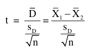
with n-1 degrees of freedom and standard error: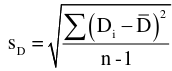
The test is inversely related to variance.
Types of Matching
- Matched Pairs (covered today)
- Categorical Matching (unmatched analysis, stratified or regression)
- Stratify cases, then find equal number of controls for each category (or equal multiple).
- Caliper Matching
- Only for continuous variables
- Similar to categorical but not the same
- Nearest Neighbor
- Select 'closest' control as match
- May have minimum match criteria
Matching in Follow-Up Study
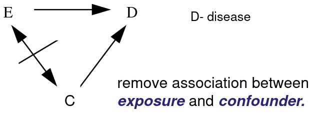
Remove Confounding (C) in the study sample between Exposed (E) and unexposed by matching on the potential confounders.
There are 4 possible combinations of outcomes in exposed and unexposed groups: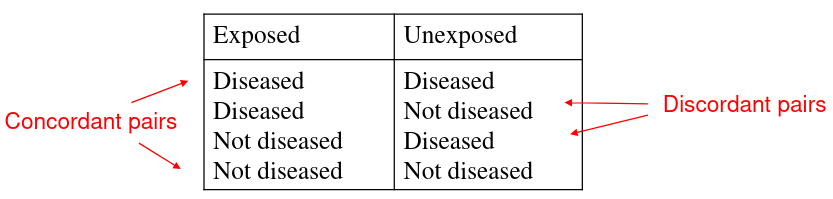
Corncordant pairs have the same outcome between pairs, and opposite in discordant pairs.
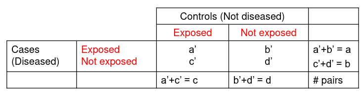
An example presentation for matching 2x2 tables: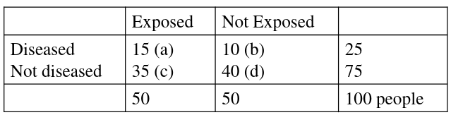
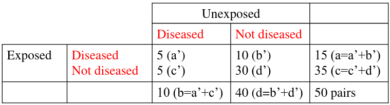
Notice the column and cell totals now equal the value of cells a,b,c,and d in the original table.
In the paired follow-up study table we would calculate the Relative Risk Ratio: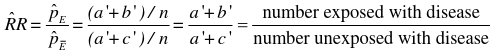
If we take the Risk Ratio of both the above tables, we find they are both the same (1.5).
Also, the confidence interval for RR in a follow up would be: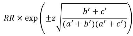
Matching in Case-Control Study
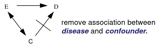
Remove Confounding (C) in the sample study between cases and controls by matching on potential confounders where for each case we select a control with the same values for the confounding variables.
For case control studies we set up our pairs differently:
And this also result in a different estimate of Odds Ratio: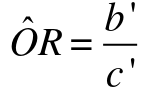
And likewise the confidence interval would be
OR x exp(+/- Z*sqrt(1/b' + 1/c')
ORs in Case-Control studies will not be the same if ignoring matching. This is unlike the situation for RR, where the point estimate is the same whether considering the matching or not.
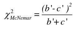
The McNemar Test
The McNemar Test is a non-parametric test for paired nominal data. It is a chi-square distribution and can be used for retrospective case-control or follow-up studies. It assumes:
- The two groups are mutually exclusive
- A random sample
H0: The proportion of some disease is the same in participants with exposure and those without exposure (RR=1)
Ha: The proportion of some disease is not the same in participants with exposure and those without exposure (RR != 1)
 with df = 1
Matched Analyses and Mantel-Haenszel
Mantel-Haenszel methods applied to strata established by matched sets are equivalent to the conventional matched methods. Works for Cohort (Follow-Up) and case-control studies. When the matched pair is a stratum, we carry out the MH method on each pair.
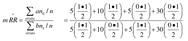
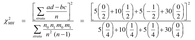
So from the example above, if we calculated 50 strata for 50 matched pairs, we would end up with 50 tables:
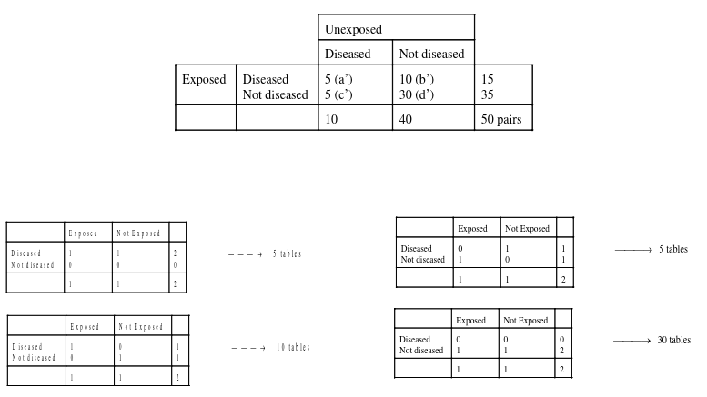
And then we apply the mRR and MH to each of the 50 strata to obtain the McNemar result.
Code
Assuming our dataset already contains matched pairs:
### Matched pairs can be analyzed using the Mantel-Haenszel method.
### Each matched pair is treated as a separate stratum
mantelhaen.test(pairs$exposed, pairs$diseased, pairs$match, correct=FALSE)

# table of pairs:<br>
table(exposed.d , unexposed.d)

### Analyze data with mcnemar.test()
mcnemar.test(table(exposed.d , unexposed.d), correct=FALSE)
mcnemar.test(table(exposed.d , unexposed.d))