Two-Way ANOVA and Power Calculations
We've learned about One-Way Analysis of Variance (ANOVA) previously, it is a regression model for one continuous outcome and one categorical variable. It allows us to compare the means of the groups to detect significant differences.
A one-way fixed-effects ANOVA is an extension of the two-sample t-test. There are factors, categorical variables, and levels, individual groups of the factor which represent different populations. Balanced design contain the same number of individuals in each level. This is a special case of linear regression.
Assumptions of one-way ANOVA:
- The data are random samples from k independent populations
- Within each population the dependent variable is normally distributed
- The observations are independent
- The population variance of the dependent variable is equal in all groups (homoscedasticity)
H0: The mean level is independent of the factor
Ex. The mean testosterone level is independent of smoking history. A conclusion might be "there is evidence that testosterone level is significantly different in at least two of the smoking history groups.
We test the hypothesis by decomposing the overall variance into "explained" and "residual" variances and comparing them.
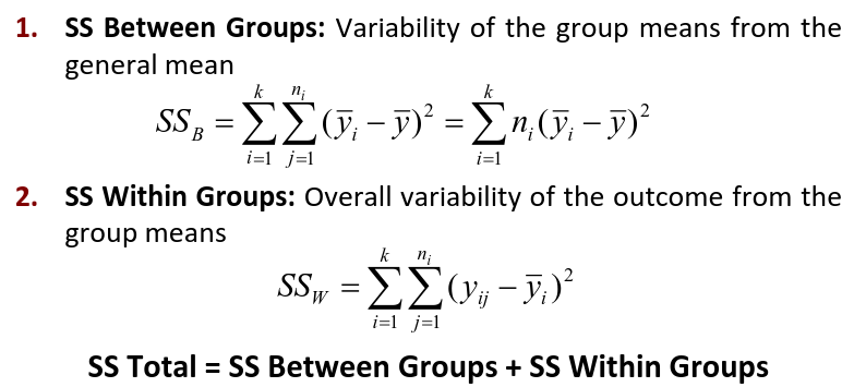
Where N is the total sample size and k is the number of groups
SSB represents the variability due to the treatment effect. SSW represents the residual variability.
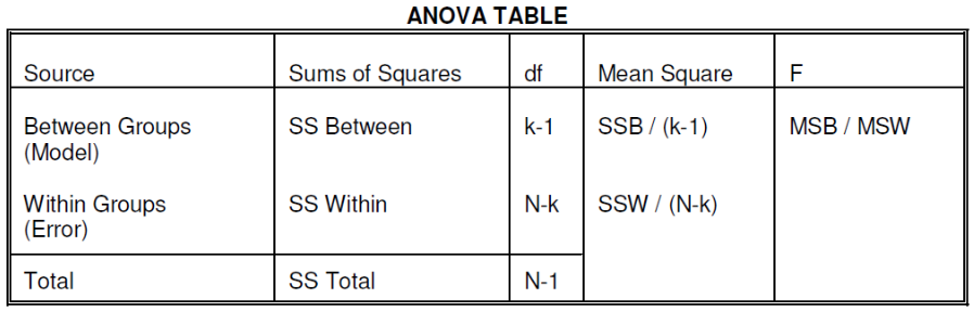
We compare the F statistic to the critical value of F with [(k - 1), (N - k)] degrees of freedom to test the null hypothesis of equal means.
Multiple Comparisons Procedures
To find which means are different from each other we should make all pairwise comparisons (k*(k-1)/2). This introduces the multiple tests issues and increases likeliness of type I and II errors. Multiple comparison procedures take into account the total number of comparisons being made by lowering the significance level for each test so that the overall significance level is still fixed at some level alpha.
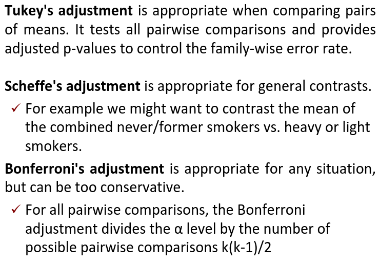
All of these adjustments are appropriate when comparing pairs of means. Tukey's is the most powerful and provides exact p-values when the group sizes are equal. Scheffe's procedure is more powerful than Bonferroni's procedure, in general.
We can also write ANOVA as a linear regression model where the parameter alpha_i are the group effects (difference of effect between group i and group 1)
Two Way ANOVA
Two way ANOVA is a regression model for one continuous outcome and two categorical variables. We analyze two-way ANOVA experiments using additive and interaction models.
An experiment may also contain replication, for example consider the following tables: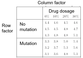
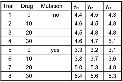
Both are the same data where the two factors are drug dosage and mutation, and we have 3 replications.
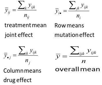
We can create summaries of the means: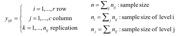
Possible Models
Interaction model: The effect of each factor changes as the other factor levels vary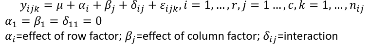
Additive model: The effect of each factor doesn't change as the other factor levels vary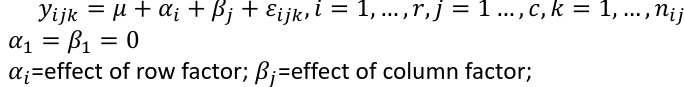
We test different models using ANOVA to look at the global effect of the factors
R Code
####### Two-way ANOVA
##### drug dataset
drug <- read.csv("anova.csv", header=T)
drug

hbf <- c(t(drug[,3:5]))
SNP <- c(rep("No",12), rep("Yes", 12))
Drug <- c(rep(0,3), rep(10,3), rep(20,3), rep(30,3),
               rep(0,3), rep(10,3), rep(20,3), rep(30,3))
data.drug <- data.frame(hbf,SNP, Drug)
head(data.drug)

### summaries
overall.mean <- mean(hbf); overall.mean
drug.means <- tapply(hbf, Drug, mean); drug.means
snps.means <- tapply(hbf, SNP, mean); snps.means
cell.means <- tapply(hbf, interaction(Drug,SNP), mean); cell.means

dim(cell.means) <- c(4,2); cell.means
cell.means <- data.frame(cell.means)
row.names(cell.means) <- levels(factor(Drug))
names(cell.means) <- levels(factor(SNP))
cell.means

## Visualization
#install.packages("gplots")
library(gplots)
plotmeans(hbf~Drug, data=data.drug,xlab="Drug",
		ylab="HbF",  main="Mean Plot\n with 95% CI")
plotmeans(hbf~SNP, data=data.drug,xlab="SNP",
		ylab="HbF",  main="Mean Plot\n with 95% CI")
plotmeans(hbf~interaction(Drug,SNP), data=data.drug,
		xlab="SNP",  connect=list(1:4,5:8),ylab="HbF",
          	main="Interaction Plot\nwith 95% CI")

interaction.plot(factor(Drug), factor(SNP), hbf, type="b",
		xlab="Drug", ylab="hbf", main="Interaction Plot")


### two-way anova with balanced design
mod <- aov(hbf~as.factor(Drug)*SNP, data=data.drug)
summary(mod)
table(mod$fitted.values)

# TukeyHSD(mod)
mod <- lm(hbf~as.factor(Drug)*SNP, data=data.drug)
summary(mod)
anova(mod)
table(mod$fitted.values)

##### Exercise with balance design

mod.a <- aov(hbf~as.factor(Drug)*SNP, data=data.drug)
summary(mod.a)		# anova(mod.a)
mod.lma <- lm(hbf~as.factor(Drug)*SNP, data=data.drug)
anova(mod.lma)

mod.b <- aov(hbf~SNP*as.factor(Drug), data=data.drug)
summary(mod.b)		# anova(mod.b)
mod.lmb <- lm(hbf~SNP*as.factor(Drug), data=data.drug)
anova(mod.lmb)


##### Exercise with unbalance design
data.drug.1 <- read.csv("data.drug.1.csv", header=T)
mod.1a <- aov(hbf~as.factor(Drug)*SNP, data=data.drug.1)
summary(mod.1a)
mod.1lma <- lm(hbf~as.factor(Drug)*SNP, data=data.drug.1)
anova(mod.1lma)


mod.1b <- aov(hbf~SNP*as.factor(Drug), data=data.drug.1)
summary(mod.1b)
mod.1lmb <- lm(hbf~SNP*as.factor(Drug), data=data.drug.1)
anova(mod.1lmb)