GLM for Multinomial Outcomes
Multinomial outcomes are much akin to binomial outcomes, with added complexity due to outcomes with more than 2 levels. In such cases it can be difficult to determine an 'order' to the outcomes.
Log-linear models can be used for analysis of this type of data. For example, if we have some distribution where πij represents the probability that the ith individual falls under the jth category. Assuming the response categories are mutually exclusive:
For each individual i; That is the probabilities add up to 1 for each individual, so we only have J - 1 probability parameters.
Multinomial Distribution
This is an extension of the binomial distribution involving joint distributions. Specifically each trial can result in any of the k events (E1, E2 ... Ek), each with its own respective probabilities. The probability that in n trials we observe Y1 of the E1 outcomes, y2 of the R2 outcomes ... and yk of the Rk outcomes in n independent trials is:![]()
with y1 + y1 .. + yk = n and the probabilities summing to 1
The multinomial term: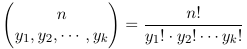
represents the number of possible divisions of n distinct objects into k distinct groups of sizes y1, y2... yk
Consider an example with k = 3 (three possible outcomes):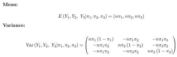
The multinomial distribution model counts are negatively correlated; The dispersion parameter is φ = 1
The binomial distribution can be thought of as a particular case of the multinomial distribution with k = 2. We want models for the mean of the response or equivalently for the probabilities, where the probabilities depend on a vector of covariates.
Link Function - Generalized Logits
Perhaps the simplest approach to the Multinomial regression is to designate one of the response categories as the reference category and calculate the log-odds for all other categories relative to the reference. For the binomial example, the reference cell is often the 'non-event' category.
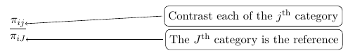
So for a multinomial with J categories there are J - 1 distinct odds. For example, in a case with 3 response categories we could use the last category as the reference and hence get 2 generalized odds also called generalized logits: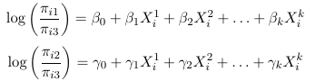
This is kind of like running 2 separate logistic regressions and estimating two separate sets of parameters, but it is a single model and all parameters are estimated by the MLE.
We can solve for the probabilities as a function of the slope parameters (beta and gamma):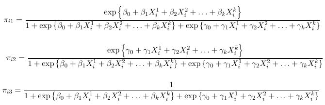
Thus, for a multinomial response with J categories, the J - 1 generalized logits are: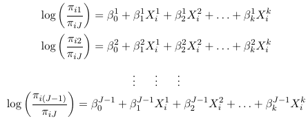
And then maximum likelihood can be used to estimate all parameters. For the intercept and each predictor, we will be estimating J - 1 parameters. Note that it really makes no difference which category is the reference, as we can always convert from one model formulation to another.
Interpretation
The generalized odds of having a response j relative to J are: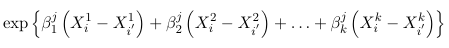
times higher for an individual with characteristics Xi1, Xi2, Xi3... Xik than for a individual with characteristics Xi'1, Xi'2, Xi'3... Xi'k. In particular, keeping X2 through Xk constant for each increase of one unit in X1 the odds of having a response j relative to J changes by a multiplicative factor of exp(beta1j)
Multinomial Ordinal Responses
Consider a multinomial random varaible Yi that may take one of J outcomes, assume there is a natural order from 1 to J. The probability falls into category j or lower is fij = P(Yi <= j), also called the cumulative probabilities.
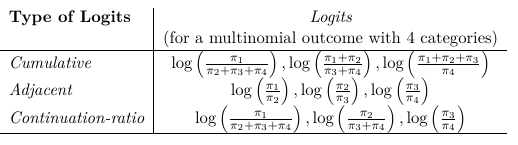
When we have a clear order between categories several alternative regression models are available. We could use generalized logits model but it ignores the order of the levels and this have diminished power. The drawback of multinomial logits compared to general multinomial logits is that assumptions imposed may not be valid. We consider 3 types of models in which the order of the factors is relevant:
- Cumulative Logits models - most widely used

- Adjacent-Categories Logits models

- Continuation-Ratio Logits models
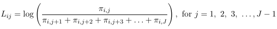

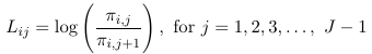

Once one decides what type of logit to use, we construct the logits model with the following identities:

Where Lij are one of the 3 logit types considered above.
These models assume separate intercept for each logit j and the same coefficients for the covariates. The intercept parameters (alpha) are also called cut-point parameters and follow the order of the ordered categorical outcome.
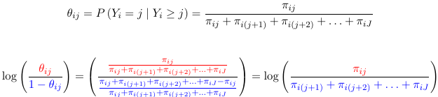
Cumulative Logits Models
A model for the cumulative logits Lij is a model for a binary outcome in which success is defined as any category <= j. Note that the cumulative logits model for a multinomial outcome is not equivalent with J-1 classical logit models. We can also write it as: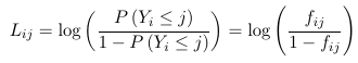
The model also assumes for 2 individuals the relative odds of being at or below a given cut-point (j) on the outcome is independent of the choice of cut-point (j); Meaning separate intercepts for each j of the ordered categorical outcome and the same slope for each predictor. As a consequence of this two individuals i and i' are independent of j:
Because of this, this model is also called the proportional odds model.
The proportional cumulative odds model will estimate a common value for two odds ratios. While the calculations might not always be exactly equal, the estimated values should suggest proportional odds. This can be tested in a logistic model in SAS.
Interpretation
The intercept alpha represents the log odds of having a response <= j when all explanatory variables are 0.
The slope is the increase in logodds of having a response <= j for an individual with characteristics X1 ... Xk than for an individual with characteristics X'1 ... X'k. Particularly it means keeping X2 ... Xk constant each increase of X1 by one unit increases the log odds by beta.
The odds of having a response <= j is:
Each explanatory variable specific odds ratio can be interpreted as the effect of that variable on the ODDS of being in a lower rather than higher category.
Adjacent Categories Logits Models

The same linear combination of predictors applies simultaneously for all J-1 pairs of adjacent response categories. The only thing that varies is the intercept.
Sometimes adjacent logits are defined equivalently as: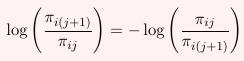
In SAS PROC CATMOD defines the adjacent logits as the former, log(πi(j+1) / πij)
Parameter Interpretation
For two individuals the relative odds of being in category j instead of j+1 is independent of choice of cut-point. Thus for 2 individuals i and i':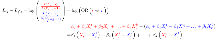
Again, independent of j. That is the ratio of odds of a response j instead of j+1 comparing two groups are the same for every j.
The adjacent odds are exp(![]() ) times higher for an individual with characteristics X1 ... Xk than for an individual with characteristics X'1 ... X'k. Particularly it means keeping X2-Xk constant each increase of X1 by one unit increases the adjacent odds by exp(beta).
) times higher for an individual with characteristics X1 ... Xk than for an individual with characteristics X'1 ... X'k. Particularly it means keeping X2-Xk constant each increase of X1 by one unit increases the adjacent odds by exp(beta).
If we allow the slopes to vary, the proportional odds assumption does not hold.
Continuation Ratio Logits Model
![]()
The same linear logit effect applies simultaneously for all J-1 continuation-ratio logits, the only coefficients that vary are the intercepts.
Let ![]() be the probability of the response in the jth category given that we know the response is >= j.
be the probability of the response in the jth category given that we know the response is >= j.
In other words the continuation-Ratio logits are the ordinary logits of the conditional probabilities of the response being j given that the response is at least j.
Alternatively, some books define the continuation-Ratio logits as:
This is not included in SAS, needs to be programmed.
This model might be more appropriate when ordered categories represent a progression of stages.
Parameter Interpretation
Based on the model for two individuals, the relative odds of being classified in the category j given it is classified in a a >= j category is independent of the choice of cut-point. For two individuals i and i':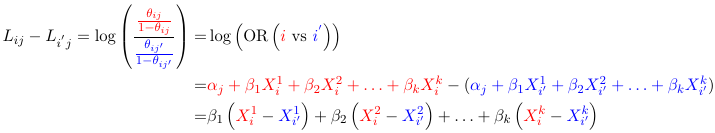
That is the odds of being classified in the jth category given it is classified in a category >= jth comparing two groups is the same for every j.
The continuation ratio odds are exp(![]() ) times higher for an individual with characteristics X1 ... Xk than for an individual with characteristics X'1 ... X'k. Particularly it means keeping X2-Xk constant each increase of X1 by one unit increases the continuation odds by exp(beta).
) times higher for an individual with characteristics X1 ... Xk than for an individual with characteristics X'1 ... X'k. Particularly it means keeping X2-Xk constant each increase of X1 by one unit increases the continuation odds by exp(beta).
SAS Code
SAS is a series of crappy procedures with no coherent structure or consistency.
/* Contraceptive data 1=Sterilization,2=Other, 3=None*/
data contra;
input age method count ref total;
cage=age-4;
agesq=cage**2;
elsn=log((count/total)/(ref/total));
datalines;
1 1   3 232 296
1 2  61 232 296
1 3 232 232 296
2 1  80 400 617
2 2 137 400 617
2 3 400 400 617
3 1 216 301 648
3 2 131 301 648
3 3 301 301 648
4 1 268 203 547
4 2  76 203 547
4 3 203 203 547
5 1 197 188 435
5 2  50 188 435
5 3 188 188 435
6 1 150 164 338
6 2  24 164 338
6 3 164 164 338
7 1  91 183 284
7 2  10 183 284
7 3 183 183 284
;
run;

goptions reset=all ftext='arial' htext=1.2 hsize=9.5in vsize=7in aspect=1 horigin=1.5in vorigin=0.3in ;
goptions device=emf rotate=landscape gsfname=TempOut1 gsfmode=replace;
filename TempOut1 "C:\Projects\BS853\Class 7\contraceptive.emf";

axis1 label=('AGE') minor=none order=(1 to 7 by 1) value=(tick=1 '15-19' tick=2 '20-24' tick=3 '25-29' tick=4 '30-34' tick=5 '35-39'
tick=6 '40-44' tick=7 '45-49') ;
axis2 label=(a=90 'Log Generalized Logit (None as reference)') minor=none ;
symbol1 v=circle i=j cv=red ci=blue;
symbol2 v=dot i=j cv=green ci=magenta;
legend1 value=('Sterilization' 'Other') label=('Method') ;

proc gplot data=contra;
plot elsn*age=method/vaxis=axis2 haxis=axis1 legend=legend1;
where method in (1,2);
run;

/*Model 1*/
options ls=97 nodate pageno=1;
title1 'Contraceptive data';
title2 'Using PROC LOGISTIC - AGE categorical';
proc logistic data=contra order=data;
freq count;
class age method/param=glm;
model method=age/link=glogit;
contrast '1 vs 2'  age 1 -1 0 0 0 0 0 /estimate=exp;
run;

/*Using Genmod*/
title2 'Using PROC GENMOD- AGE categorical';
proc genmod data=contra  order=data;
 class method age;
 model count = method age method*age/dist=p;
run;

title2 'Using PROC CATMOD- AGE categorical';
proc catmod data=contra order=data;
weight count;
model method=age;
run;

/*Model 2 */
title2 'Using PROC LOGISTIC - continuous age linear effect';
proc logistic data=contra order=data;
freq count;
model method=cage/link=glogit;
run;

title2 'Using PROC CATMOD - continuous linear effect';
proc catmod data=contra order=data;
direct cage;
weight count;
model method=cage;
run;

/*Model 3*/

title2 'Using PROC LOGISTIC  - continuous age linear and quadratic effects';
proc logistic data=contra order=data ;
freq count;
model method=cage agesq/link=glogit ;
output out=aa(where=(_level_ in (1,2) and method in (1,2) and method=_level_)) xbeta=pred;
run;

title2 'Using PROC CATMOD - continuous age linear and quadratic effects';
proc catmod data=contra order=data;
direct cage agesq;
weight count;
model method=cage agesq;
run;

/*Using Genmod*/
title2 'Using PROC GENMOD - continuous age linear and quadratic effects';
proc genmod data=contra;
 class method age;
 model count = method age method*cage method*agesq/dist=p;
run;

filename TempOut1 "C:\Projects\BS853\Class 7\contraceptivepred1.emf";

axis1 label=('AGE') minor=none order=(1 to 7 by 1) value=(tick=1 '15-19' tick=2 '20-24' tick=3 '25-29' tick=4 '30-34' tick=5 '35-39'
tick=6 '40-44' tick=7 '45-49') ;
axis2 label=(a=90 'Log Generalized Logit (None as reference)') minor=none ;
symbol1 v=circle i=j cv=red ci=blue;
symbol2 v=dot i=j cv=green ci=magenta;
legend1 value=('Observed' 'Predicted') label=('') ;
title1 h=1.2 'Predicted vs. Observed For Method=Sterilization';
proc gplot data=aa;
plot elsn*age pred*age/vaxis=axis2 haxis=axis1 overlay  legend=legend1;;
where method=1;
run;

/* Using SGplot */
ods listing gpath="Z:/Documents/BS853/Spring 2019/Class 6/";
ods graphics / reset width=600px height=400px  imagename="Pred1" imagefmt=gif;
title1 h=1.2 'Predicted vs. Observed For Method=Sterilization';
proc sgplot data=aa cycleattrs;
 yaxis grid label="Log Generalized Logit (None as reference)";
  xaxis grid label="Age";
   series  x=age y=elsn / lineattrs = (pattern=solid thickness=3)
           legendlabel = "Observed Data" name= "elsn";
   scatter x=age y=elsn/ markerattrs=(symbol=circlefilled size=10  color=orange);;
   series  x=age y=pred / lineattrs = (pattern=solid thickness=3)
           legendlabel = "Model" name= "pred";
   scatter x=age y=pred/ markerattrs=(symbol=squarefilled size=10 color=green);
	keylegend "elsn" "pred";
where method=1;
run;

filename TempOut1 "C:\Documents and Settings\doros\My Documents\Projects\BS853\Class 7\contraceptivepred2.emf";

title1 h=1.2 'Predicted vs. Observed For Method=Other';
proc gplot data=aa;
plot elsn*age pred*age/vaxis=axis2 haxis=axis1 overlay  legend=legend1;;
where method=2;
run;

/* Using SGplot */
ods listing gpath="Z:/";
ods graphics / reset width=600px height=400px  imagename="Pred2" imagefmt=gif;
title1 h=1.2 'Predicted vs. Observed For Method=Other';
proc sgplot data=aa cycleattrs;
 yaxis grid label="Log Generalized Logit (None as reference)";
  xaxis grid label="Age";
   series  x=age y=elsn / lineattrs = (pattern=solid thickness=3)
           legendlabel = "Observed Data" name= "elsn";
   scatter x=age y=elsn/ markerattrs=(symbol=circlefilled size=10  color=orange);;
   series  x=age y=pred / lineattrs = (pattern=solid thickness=3)
           legendlabel = "Model" name= "pred";
   scatter x=age y=pred/ markerattrs=(symbol=squarefilled size=10 color=green);
	keylegend "elsn" "pred";
where method=2;
run;


/*Schoolchildren learning style preference and School program*/
/* styles 1=Self,2=Team,3=Class*/
data school;
 do style=1 to 3;
input school program $ count @@;
output;
end;
cards;
1 Regular 10 1 Regular  17 1 Regular  26
1 After    5 1 After    12 1 After    50
2 Regular 21 2 Regular  17 2 Regular  26
2 After   16 2 After    12 2 After    36
3 Regular 15 3 Regular  15 3 Regular  16
3 After   12 3 After    12 3 After    20
run;

title1 'Estimating parameters using contrast statement';
options ls=97 nodate pageno=1;
ods select contrastestimate;
proc logistic data=school order=data;
freq count;
class school program/param=glm;
model style=school program /link=glogit;
contrast 'reg vs. after' program -1 1/estimate=exp;
run;

/*Consider data on association of cumulative incidence of
pneumoconiosis and years working at a coalmine.*/

data ph;
do type=1 to 3;
input age count @@;
output;
end;
cards;
1 218 1 13 1 12
2  71 2 25 2 32
run;

options ls=97 nodate pageno=1;
title1 'Cumulative Logit models - PROC GENMOD';
  proc genmod data=ph order=data descending;
      freq count;  /*<-group data*/
      class age;
      model type = age / dist=multinomial link=cumlogit type3;
      estimate 'LogOR12' age -1 1 / exp;
   run;
title1 'Cumulative Logit models - PROC LOGISTIC';
     proc logistic data=ph order=data descending;
      freq count;
      class age/param=glm;
      model type = age;
     contrast 'LogOR12' age -1 1 / estimate=exp;
   run;

/* Metal Impairement data - Agresti, 1990*/

proc import datafile="Z:\Documents\BS853\Spring 2015\Class 6\impair.xls"
out = mimpair replace;
run;

options ls=97 nodate pageno=1;
title1 'Cumulative Logit models - PROC GENMOD';
  proc genmod data=mimpair rorder=data;
      model level = SES EVENTS/ dist=multinomial link=cumlogit type3;
      estimate 'LogOR12' SES 1  / exp;
   run;

title1 'Cumulative Logit models - PROC LOGISTIC';
    proc logistic data=mimpair order=data ;
     class level;
      model level = SES EVENTS ;
      contrast 'LogOR12' SES 1  / estimate=exp;
   run;
The RESPONSE statement in PROC CATMOD defines the function of the response probabilities (the link function) that we want to model as linear combinations of the predictors. Operations in the RESPONSE statement should be read right to left with the vector of observed response probabilities understood to be the right-most quantity. The rows of the matrices are separated by commas.
The _RESPONSE_ variable is a categorical variable with seperate levels for each of the logits.
/*satisfaction with THR and hospital volume and year of surgery.*/
proc format ;
  value vol 1='High' 0='Low';
run;
data thr;
input  year highvol satisf count total123 total12;
if satisf=1 then cuml1=log(count/(total123-count));
if satisf=2 then cuml2=log(total12/(total123-total12));count;
format highvol vol.;
datalines;
1         0         1        84
414       315
1         0         2       231       414       315
1         0         3        99
414       315
1         1         1       473      1059       966
1         1         2       493
1059       966
1         1         3        93      1059       966
2         0         1       150
614       497
2         0         2       347       614       497
2         0         3       117
614       497
2         1         1       332       781       719
2         1         2       387
781       719
2         1         3        62       781       719
3         0         1       257
1380      1146
3         0         2       889      1380      1146
3         0         3       234
1380      1146
3         1         1       571      1476      1364
3         1         2       793
1476      1364
3         1         3       112
1476;
1364run;

options pageno=1 nodate ps=57 ls=91;
title1 'Adjacent Logits models for THR';
proc catmod data=thr;
  weight count;
  response ALOGIT;
  model satisf= _response_ highvol year;
run;
quit;


/* let the effect of year vary with the cutpoint*/
title1 'Adjacent Logits models for THR - with coefficents dependent on the level of satisfcation';
proc catmod data=thr ;
  weight count;
  response ALOGIT;
  model satisf= _response_ highvol _response_|year;
run;
quit;


/* number of hip fractures by race age and BMI */
/* n=0 then no hip fractures, n=1 then 1 hip fractures, n=2 then more than 1 hip fractures */
data nhf;
do n=0 to 2;
input race $ age $ bmi count @@;
output;
end;
cards;
white	<=80 	1	39	white	<=80 	1	29	white	<=80 	1	8
white	<=80	2	4	white	<=80	2	8	white	<=80	2	1
white	<=80	3	11	white	<=80	3	9	white	<=80	3	6
white	<=80	4	48	white	<=80	4	17	white	<=80	4	8
white	>80 	1	231	white	>80 	1	115	white	>80 	1	51
white	>80	    2	17	white	>80	    2	21	white	>80	    2	13
white	>80	    3	18	white	>80	    3	28	white	>80	    3	45
white	>80	    4	197	white	>80	    4	111	white	>80	    4	35
black	<=80 	1	19	black	<=80 	1	40	black	<=80 	1	19
black	<=80	2	5	black	<=80	2	17	black	<=80	2	7
black	<=80	3	2	black	<=80	3	14	black	<=80	3	3
black	<=80	4	49	black	<=80	4	79	black	<=80	4	24
black	>80 	1	110	black	>80 	1	133	black	>80 	1	103
black	>80	    2	18	black	>80	    2	38	black	>80	    2	25
black	>80	    3	11	black	>80	    3	25	black	>80	    3	18
black	>80	    4	178	black	>80	    4	206	black	>80	    4	81
;
run;
options pageno=1 nodate ps=57 ls=91;
/* continuation ratio logits models*/
 title1 'Continuation-ratio Logits models for NHF using the response statement';
proc catmod data=nhf;
     weight count;
     response * 1 -1 0  0,
                0  0 1 -1  log  * 1 0 0,
                                  0 1 1,
                                  0 1 0,
                                  0 0 1;  /* p1
                                             p2
                                             p3  */
     model n=_response_ age bmi|race/  predict;
     run;
     quit;

	 /* Use second way to defining continuation ration logits */
title1 'Continuation-ratio Logits models for NHF using the response statement(2)';
  proc catmod data=nhf;
     weight count;
     response * -1 1  0 0,
                 0 0 -1 1  log  * 1 0 0,
                                  0 1 0,
                                  1 1 0,
                                  0 0 1;
     model n=_response_ age bmi|race/ prob predict;
     run;
     quit;

/* let the coefficients depend on the number of hip fracturs */
 title2 'Coefficients dependent on the number of HF';
proc catmod data=nhf;
     weight count;
     response * 1 -1 0 0,
                0 0 1 -1  log  * 1 0 0,
                                 0 1 1,
                                 0 1 0,
                                 0 0 1;

     model n=_response_|bmi _response_|age _response_|race  bmi|race/ freq;
     run;
     quit;

title1 'Adjacent Logits models for THR using the response statement';
proc catmod data=thr;
  weight count;
 response * -1  1 0,
             0 -1 1  log  * 1 0 0,
                            0 1 0,
                            0 0 1;  /* p1
                                       p2
                                       p3  */
  model satisf= _response_ highvol year;
run;
quit;

title1 'cumulative Logits models for THR using the response statement';
proc catmod data=thr;
  weight count;
 response *  1 -1 0  0,
             0  0 1 -1  log  * 1 0 0,
                               0 1 1,
                               1 1 0,
                               0 0 1;  /* p1
                                       p2
                                       p3  */
  model satisf= _response_ highvol year;
run;
quit;
title1 'cumulative Logits models for THR using Proc Logistic ';
proc logistic data=THR;
  class highvol year;
  model satisf= highvol year;
  freq count;
run;

/********************************************************************************/
/***               Overdispersion in binomial models                          ***/
/********************************************************************************/
DATA aggregate;
  INPUT pot total yes cultivar soil @@;
cards;
 1 16  8 0 0   2 51 26 0 0
 5 36  9 0 0   6 81 23 1 0
 9 28  8 1 0  10 62 23 1 0
13 41 22 0 1  14 12  3 0 1
17 30 15 1 1  18 51 32 1 1
 3 45 23 0 0   4 39 10 0 0
 7 30 10 1 0   8 39 17 1 0
11 51 32 0 1  12 72 55 0 1
15 13 10 0 1  16 79 46 1 1
19 74 53 1 1  20 56 12 1 1
;
run;


/* Onlyno mainscale effects- modelaggregated data'*/
options ls=97pageno=1 nodate pageno=1;ps=57 ls=91;
title1 'Only mainNo effectsScale model'';
proc logisticgenmod data=thr ;
freq count; /* <- to deal with the grouped data */
class year;aggregate;
model satisf=highvolyes/total year/aggregate= scale=n;cultivar|soil/type3 /*dist=binomial Aggregate and scale=n to get goodness of fit stats*/;
run;

/*  Onlyscale volume- mainaggregated effectdata'*/
in/* theModel model2 */
options ls=97 nodate pageno=1;
title1 'Only volumeScale effectparameter model'estimated by the scaled dispersion ';
proc logisticgenmod data=thraggregate;
model yes/total = cultivar|soil/type3 dist=binomial dscale ;
freq count;
class ;
model satisf=highvol/aggregate scale=n;
run;

/* Only volume main effect in the model */
options ls=97 nodate pageno=1;
title1 'Only volume effect model';
proc logistic data=thr ;
freq count;
class ;
model satisf=highvol;
output out=bb(where=(_level_ in (1,2) and satisf in (1,2) and satisf=_level_)) xbeta=pred;
run;

 goptions reset=all ftext='arial' htext=1.2 hsize=9.5in vsize=7in aspect=1 horigin=1.5in vorigin=0.3in ;
 goptions device=emf rotate=landscape gsfname=TempOut1 gsfmode=replace;
  		filename TempOut1 "C:\Documents and Settings\doros\My Documents\Projects\BS853\Class 7\contraceptive.emf";

filename TempOut1 "C:\Projects\BS853\Class 7\hr1.emf";

axis1 label=('Year') minor=none order=(1 to 3 by 1) value=(tick=1 '1994' tick=2 '1995' tick=3 '1996') ;
axis2 label=(a=90 'Log Cumulative Logit ') minor=none ;
symbol1  v=circle cv=red  pointlabel=(h=1.2 "#highvol");
symbol2 v=dot  cv=green  pointlabel=(h=1.2 "#highvol");;
legend1 value=('Observed' 'Predicted') label=('') ;
title1 h=1.2 'Very vs. Somewhat or Not satisfied';
proc gplot data=bb;
plot cuml1*year pred*year/vaxis=axis2 haxis=axis1 overlay  legend=legend1;;
where satisf=1;
run;
filename TempOut1 "C:\Documents and Settings\doros\My Documents\Projects\BS853\Class 7\hr2.emf";
title1 h=1.2 'Very or Somewhat vs. Not satisfied';
proc gplot data=bb;
plot cuml2*year pred*year/vaxis=axis2 haxis=axis1 overlay  legend=legend1;;
where satisf=2;
run;