Binomial Outcomes
Frequently dichotomous outcomes are used in medical studies, such as presence of a disease or exposure to some factor. The classical model does not apply outcomes that are not continuous, and many other reasons:
- The variance of the dichotomous response is not constant
- One could predict probabilities > 1 or smaller than 0
- Limited interpretation of parameters
In this section we will observe alternatives to traditional linear regression for binomial data.
Generalized Linear Model For Binomial Data
- The outcome is distributed either Bernoulli or Binomial with probability of success θ
- Link function is logit and relates to the probability of success θ to the linear predictor η = β0 +β1 X1 +
β2X2 + · · · + βk−1Xk−1 + βk Xk as follows:

- Variance function: V(θ) = θ (1 - θ)

Recall: For ordinary linear regression the distribution of outcomes is normal and the link is the identity function, and the variance is constant. For loglinear models the distribution of the outcome is Poisson, the link function is the LOG function and the variance function is the identity.
The link function is logistic because the logit function takes value between -inf to inf while the logodds is between 0 and 1.
β represents the increase in logodds for a one-unit increase in X
The coefficients can also be interpreted as probability (risk) difference. However, the change is a function of base probability:
Probit, Complementary Log-Log, and Logistic Regression
Probit regression and Complementary log-log regression are generalized linear models for the same type of data as the logistic regression, the only difference is in the choice of the link functions.
- Probit uses a link function which is the inverse of the Cumulative Distribution Functions (CDF) of a standard normal distribution
- Link function:
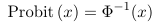
Where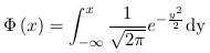
- Probit and logistic will in general give similar results in terms of significance; The advantage of logistic regression is interpretability of coefficients as OR's
- Logit and Probit haave the symmetry property, that is:
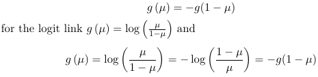
- Link function:
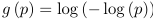
- Complementary log-log is inverse of the CDF for an extreme value distribution
- The link function:

- Does not have the symmetry property, a good choice when symmetry property does not hold.
- The link function:


Interpretation of Parameters
Note we've already seen how to interpret logodds in 806 and 852 so I will not being going into great detail here.
One neat thing is that we can express any model using shorthand. 
Where CHOL and SBP are binary variables representing levels of these measures. The shorthand equivalent: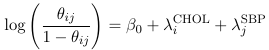
While not as informative about the levels and coefficients, it is much easier to write.
Testing Goodness of Fit and Model Selection in Logistic Regression
As in any other model we can assess the GoF by comparing the observed to the predicted. The deviance statistic (also called the Likelihood Ratio Statistic) is the GoF measure of choice for this class.
Which reduces to the following for binomial models: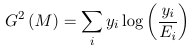
Where Ei = ni πi
The Pearson Chi-Squared Test are application for logistic regression when the data can be aggregated, or grouped into unique profiles determined by predictors. Aggregation is only possible when all predictors are categorical.
With ungrouped data the Pearson chi-square test is: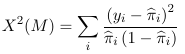
Where yi is the observed binary outcome, and pi_hat is the model estimate of probability of yi=1. This does NOT have a asymptotic chi-square distribution, but when properly standardized it follows a normal distribution
With grouped data the Pearson chi-square test is: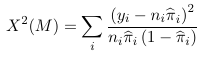
which follows a chi-square distribution
SAS Code
options ps=60 ls=89 pageno=1 nodate;

/* CHD in Framingham Study*/
proc format ;
value sbp 1='<127' 	2='127 - 146' 	3='147 - 166' 	4='167+';
value chl 1='<200'  2='200 - 219'   3='220 - 259'   4='>=260';
run;
data chd;
input Chol SBP CHD Total;
prchd=(chd+0.5)/total;
logitp=log((prchd)/(1- prchd));
format sbp sbp. Chol chl.;
cards;
1 1 2  119
1 2 3  124
1 3 3  50
1 4 4  26
2 1 3  88
2 2 2  100
2 3 0  43
2 4 3  23
3 1 8  127
3 2 11 220
3 3 6  74
3 4 6  49
4 1 7  74
4 2 12 111
4 3 11 57
4 4 11 44
;
run;


/* First, examine the relationships of incidence of CHD with Chol and SBP graphically. */
goptions reset=all ftext='arial' htext=1.2 hsize=9.5in vsize=7in aspect=1 horigin=1.5in vorigin=0.3in ;
goptions device=emf rotate=landscape gsfname=TempOut1 gsfmode=replace;
  		filename TempOut1 "C:\Documents and Settings\doros\My Documents\Projects\BS853\Class 4\Framingham.emf";
axis1 label=(h=1.5 'Cholesterol') minor=none order=(1 to 4 by  1)
value=(tick=1 '< 200' tick=2 '200 - 219' tick=3 '220 - 259' tick=4 '>= 260') offset=(1);
axis2 label=(h=1.5  a=90 'Logit(Probability)') minor=none ;

symbol1 v=none i=j ci=red line=1;
symbol2  v=none i=j ci=green line=2;
symbol3  v=none i=j ci=blue line=3;
symbol4  v=none i=j ci=magenta line=4;
title1 'Incidence of CHD with Chol and SBP';
proc gplot data=chd;
 plot logitp*chol=sbp/haxis=axis1 vaxis=axis2;
 run;
quit;
goptions reset=all;

/* Fit different Models using GENMOD and LOGISTIC*/
options ls=100 ps=60 nodate pageno=1;
title1 'Only Intercept Effect';
proc genmod data=CHD;
class CHOL SBP;
model CHD/Total=/dist=Binomial link=logit;
run;

title1 'Only Chol Effect';
proc genmod data=CHD;
class CHOL SBP;
model CHD/Total=CHOL /dist=Binomial link=logit;
run;

title1 'Only SBP Effect';
proc genmod data=CHD;
class CHOL SBP;
model CHD/Total=SBP /dist=Binomial link=logit;
run;


title1 'Only main Effects';
ods output obstats=check;
proc genmod data=CHD;
class CHOL SBP;
model CHD/Total= CHOL SBP /dist=Binomial link=logit obstats;
run;

title1 'Only main Effects - Using PROC LOGISTIC';
proc logistic data=CHD;
class CHOL SBP(ref='167+');
model CHD/Total= CHOL SBP ;
run;

title1 'Only main Effects - Continuous predictors';
ods output obstats=check;
proc genmod data=CHD;
model CHD/Total= CHOL SBP /dist=Binomial link=logit obstats ;
run;

title1 ' Saturated Model ';
proc genmod data=CHD;
class CHOL SBP;
model CHD/Total= CHOL|SBP /dist=Binomial link=logit;
run;

title1 'Only main Effects - Hosmer-Lemeshow';
ods select LackFitPartition LackFitChiSq;
proc Logistic data=CHD;
  model CHD/Total= CHOL SBP / LACKFIT;
run;

title1 'Only main Effects - R-Squared and R-Squared Nagelkerke';
ods select RSQUARE;
proc Logistic data=CHD;
  model CHD/Total= CHOL SBP / RSQUARE;
run;

 /* Logistic regression models as Log-Linear models*/
data chd2;
input chol sbp chd count @@;
datalines;
1 1 1 2  1 1 2 117
1 2 1 3  1 2 2 121
1 3 1 3  1 3 2  47
1 4 1 4  1 4 2  22
2 1 1 3  2 1 2  85
2 2 1 2  2 2 2  98
2 3 1 0  2 3 2  43
2 4 1 3  2 4 2  20
3 1 1 8  3 1 2 119
3 2 1 11 3 2 2 209
3 3 1 6  3 3 2  68
3 4 1 6  3 4 2  43
4 1 1 7  4 1 2  67
4 2 1 12 4 2 2  99
4 3 1 11 4 3 2  46
4 4 1 11 4 4 2  33
;
title1 'Logistic regression models as Loglinear models';
title2 'Model 1' ;
ods select parameterestimates modelfit;
proc genmod data=chd2;
class chol sbp chd;
model count=CHD SBP|CHOL /link=log dist=poisson obstats;
run;

ods select parameterestimates modelfit;
title2 'Model 2' ;
proc genmod data=chd2;
class chol sbp chd;
model count=CHD|SBP SBP|CHOL/link=log dist=poisson obstats;
run;

ods select parameterestimates modelfit;
title2 'Model 3' ;
proc genmod data=chd2;
class chol sbp chd;
model count=CHD|CHOL SBP|CHOL/link=log dist=poisson obstats;
run;
options ls=90;
ods select parameterestimates;* modelfit;
title2 'Model 4' ;
proc genmod data=chd2;
class chol sbp chd;
model count=CHD|CHOL CHD|SBP SBP|CHOL/link=log dist=poisson obstats;
run;

/**************************************************************/
/* Admission Data                                             */
/**************************************************************/
/* Ignoring Department */
data overall;
input sex $ yes total;
cards;
	M 1198  2691
	F   557  1835
;
/* Saturated model: with class statement*/;
ODS select modelfit ParameterEstimates;
title 'Differential admission by Gender';
proc genmod data=overall;
class sex;
model yes/total=sex/link=logit dist=bin obstats;
estimate 'overall gender' sex 1 -1/exp;
run;

proc genmod data=overall;
class sex;
model yes/total=/link=logit dist=bin obstats;
run;
/* By Department */
data one;
do Department=1 to 6;
do Sex='M', 'F';;
input yes no;
logitp=log(yes/(yes+no));
total=yes+no;
output;
end;
end;
cards;
512	313
89	19
353  	207
17     	8
120  	205
202  	391
138  	279
131 	244
53  	138
94  	299
22  	351
24  	317
;run;

/* Explain why marginally women seem to be discriminated against
   - More women apply to harder to enter colodges!!!             */

proc sql; create table a as
select department, sum(total) as total , sum(yes)/sum(total) as adminp from one group by department  order by department;
 create table b as select department, total as fem from one where sex='F' order by department;
 create table c as
 select *, fem/total as pf from a as aa, b as bb where aa.department=bb.department;
quit;

 symbol1 v=circle i=join;
 proc gplot data=c;
 plot pf*adminp;
run;


goptions reset=all ftext='arial' htext=1.2 hsize=9.5in vsize=7in aspect=1 horigin=1.5in vorigin=0.3in ;
goptions device=emf rotate=landscape gsfname=TempOut1 gsfmode=replace;
  		filename TempOut1 "C:\Documents and Settings\doros\My Documents\Projects\BS853\Class 4\admission.emf";
		symbol1 v=dot i=j ci=red;
		symbol2 v=circle i=j ci=blue;
		axis1 label=(h=1.5 'Department') minor=none order=(1 to 6 by  1)  offset=(1);
axis2 label=(h=1.5  a=90 'Logit(Rate)') minor=none ;

title1 'Admitance by Department and Sex';
proc gplot data=one;
plot logitp*Department=sex/vaxis=axis2 haxis=axis1;
run;

title1 'Saturated Model';
proc genmod data=one;
class department sex;
model yes/total=sex|department/dist=b link=logit;
run;

title1 'Only main effects Model';
proc genmod data=one;
class department sex;
model yes/total=sex department/dist=b link=logit;
run;

title1 'Only Sex Model';
proc genmod data=one;
class department sex;
model yes/total=sex/dist=b link=logit;
estimate 'l' sex 1 -1/exp;
run;

title1 'Only Department effects Model';
proc genmod data=one;
class department sex;
model yes/total=department/dist=b link=logit;
run;

ods select estimates;
title1 'Estimated ODDS Ratio (F vs M) in each Department';
proc genmod data=one;
class department sex;
model yes/total=sex|department/link=logit dist = bin covb;
estimate 'sex1'  sex 1 -1  department*sex 1 -1 0  0 0  0 0  0 0  0 0  0    /exp ;
estimate 'sex2'  sex 1 -1  department*sex 0  0 1 -1 0  0 0  0 0  0 0  0    /exp ;
estimate 'sex3'  sex 1 -1  department*sex 0  0 0  0 1 -1 0  0 0  0 0  0    /exp ;
estimate 'sex4'  sex 1 -1  department*sex 0  0 0  0 0  0 1 -1 0  0 0  0    /exp ;
estimate 'sex5'  sex 1 -1  department*sex 0  0 0  0 0  0 0  0 1 -1 0  0    /exp ;
estimate 'sex6'  sex 1 -1  department*sex 0  0 0  0 0  0 0  0 0  0 1 -1    /exp ;
run;

/* Modeling Trends in Proportions */
data refcanc;
do age=1 to 4;
input cases ref;
total=cases+ref;
output;
end;
cards;
26	20
4	7
3	10
1	11
;
run;

/* only intercept */
title1 'Only Intercept model';
proc genmod data=refcanc;
class age;
model cases/total=;
run;

/* Saturated model */
title1 'Saturated model';
proc logistic data=refcanc;
class age;
model cases/total=age;
run;
title1 'Linear trend model';

proc logistic data=refcanc;
model cases/total=age;
run;