Interim Analysis and Data Monitoring
Clinical trials are often longitudinal in nature. It is often impossible to enroll all subjects at the same time, so it can take a long time to complete a longitudinal study. Over the course of the trial one needs to consider administrative monitoring, safety monitoring and efficacy monitoring.
Efficacy monitoring can be performed by taking interim looks at the primary endpoint data (prior to all subjects being enrolled or all subjects completing treatment). This is because:
- It potentially stops the trial early if there is convincing evidence of benefit or harm of the new product
- It potentially stops the trial for futility, in other words the chance of significant beneficial effect by the end of the study is small given observed data
- Re-estimate final sample size required to yield adequate power to obtain a significant result
Interim analysis evaluates for early efficacy, early futility, safety concerns, or adaptive design with respect to sample size or power.
Group Sequential Design
A common type of study design for interim analysis is GSD, in which data are analyzed at regular intervals.
- Determine a priori the number of interim "looks"
- Let K = # of total planned analyses including final (K >= 2)
- For simplicity, assume 2 groups and that subjects are randomized in a 1:1 manner
- After every n = N/K subjects are enrolled and followed for a specific time period, perform an interim analysis on all subjects followed cumulatively
- If there is a significant treatment difference at any point, consider stopping the study
Due to multiple testing the probability of observing at least one significant interim result is much greater than the overall α = .05, as a result the interim analyses should NOT be performed using the family-wise error rate. The data at each interim analysis contains data from the previous interim and thus are not independent.
Equivalently we would have K critical values for each interim:
- First interim analysis compare test statistic to critical value Z1 |> c1. If significant then stop the trial.
- Second interim analysis compare test statistic to critical value Z2 |> c2. If significant stop the trial
- ...
- Final analysis compare test statistic to critical value Xk |> ck.
Pocock Approach (1977)
Derives constant critical values across all stages to maintain the overall significance level at .05. The critical value depends on the number of interim analyses, but is the same for each interim look.
Ex. When K=5, Z critical value = 2.413 for each interim and the final analysis. When K=4, Z critical value = 2.361.
O'Brien-Fleming Approach (1979)
Proposed sequential testing procedure that has critical values (in absolute value) decrease over the stages. Z critical value depends on total number of interim analyses and the stage of the interim analysis. The critical Z value depends on the total number of interim analyses and the stage of the interim analysis.
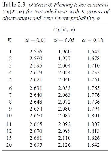
Ex. For K = 5 after after 200 subjects completed:
- C5 = 2.040 a constant determined by O'Brien-Fleming)
- First look critical value is: sqrt(5/1)*2.04 = 4.56
- Second look critical value: sqrt(5/2)*2.04 = 3.23
- ...
- Critical value final look: sqrt(5/5)*2.04 = 2.04
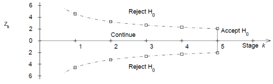
This makes it more difficult to declare superiority at "earlier" looks, but does lose much of the original alpha at the final look. This is more conservative than Pocock and the recommended approach by the FDA on their 2010 Guidance on Adaptive Designs.
Controlling the Overall Significance Level
Issues with group sequential procedures:
- Need to specify a priori for the number of planned interim analyses
- The timing of interim analyses is generally not exact calendar time but "information time" (i.e. based on sample size or number of events)
- Assumes interim analyses performed after every n subjects complete follow-up (or y events occur)
- Difficult to schedule formal review procedures for interim analyses after every n subjects (or y events); may want to allow more flexibility in scheduling
- So the main issue is: How do we allow for more flexibility for unscheduled interim analysis?
Alpha-Spending
From Lan and DeMets (1983) Biometrika: Adjust teh levels via an "alpha-spending function". Think of it like each analysis spends a bit of the alpha power.
- α(s) denotes alpha spending function.
- s = proportion of information (sample size or events) accrued
- s = 0 at the start of the study (0% information); α(0) = 0
- s = 1 is the end of the study (100% information); α(1) = 1
- α(sk) proportion of Type 1 error one is willing to spend up to time k
- Not a significance level