Multiple Imputation and Weighting Methods

If no missing data is present our statistical methods provide valid inference only if the following assumptions are met:

• For Generalized Estimating Equations, the mean function is correctly specified
• For likelihood-based methods, the probability density function including the mean and variance are correctly specified

Missing data can seriously compromise inferences from randomized clinical trials, especially when handled incorrectly, but inference is still possible with the correct methods.

Missing values in longitudinal studies may occur intermittently when individuals miss one or more planned visits, or drop out early.

Types of Missing Data

• Missing Completely at Random (MCAR) - Missingness is independent of both observed and unobserved data. More formally, the probability of missing data in Y is unrelated to the value of Y itself or any other variable X. However, it does allow for the possibility that missingness is Y is related to missingness in some other variable X.
  • Ex. In determining predictors of income, MCAR assumption would be violated if people who reported income were on average younger than the people who did report it.
• Missing at Random (MAR) - Missingness is independent of missing responses after controlling for other variables X. Formally: P(Y missing | Y,X) = P(Y missing | X)
  • Ex. The MAR assumption is satisfied if the probability of missing data on income depended on a person's age, but within each age group the probability of missing income was unrelated to income. Obviously, this cannot be tested as we do not know the missing values of the data.
• Missing Not at Random (MNAR) - Missing value depend on unobserved values.
  • Ex. High income people are less likely to report their income.
  • Also referred to as non-ignorable missing or informative dropout

Multiple Imputation

Imputation is substituting each missing value with a reasonable guess, which can be done using a variety of methods. In multiple imputation, imputed values are drawn from a distribution so they inherently contain some variation. Thus, it addresses shortcomings of single imputation by introducing an additional form of error based on variation in the parameter estimates across imputation called between imputation error. Since this is a simulation-based procedure, the purpose is not to re-create the individual missing values as close as possible to the true ones, but to handle missing data to achieve valid inference.

It involves 3 steps:

1. Run an imputation model defined by the chosen variables to create imputed data sets. In other words, the missing values are filled in m times to generate m complete data sets.
   • The standard is m = 10
   • Choosing the correct model requires considering:
     • Which variables have missing values?
     • Which has the largest proportion of missing values?
     • Are there patterns to the missingness?
       • Monotone (dropouts in longitudinal studies) or arbitrary
2. Perform an analysis on each of the m completed data sets by using a BY statement in conjunction with an appropriate analytic procedure (MIXED or GENMOD in SAS)
   • Parameter estimates, standard errors, etc. should be considered
3. The parameter estimates from each imputed data set is combined to get a final set of parameter estimates

Pros: Same properties as ML but removes limitations and can be used with any kind of data or software. When the data is MAR, multiple imputation can lead to consistent, asymptotically efficient and asymptotically normal estimates.

Cons: It is challenging to use successfully. It produces different estimates every time.

Regression-Based Imputation

Particularly with monotone missingness, we can fit a linear regression model to predict missing values Y.

1. Randomly draw from a chi-squared distribution with (N_j - q) degrees of freedom where N_j is the number of subjects who haven't dropped out at the j^th occasion and q is the number of covariates used to predict Y.
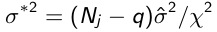
2. Calculate the residual variance of the k^th draw:
   

   

   $$\(sigma^2 = (N_j - q) \hat{ \hat\sigma^2 / \chi^2 }$$
   
   
3. When \(a \ne 0\), there are two solutions to \(ax^2 + bx + c = 0\) and they are
   $$x = {-b \pm \sqrt{b^2-4ac} \over 2a}.$$
4. Randomly draw regression parameters γ from a multivariate distribution N(γ, Cov(γ)) where:
   

   

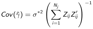
5. Draw e from N(0,  σ²), where σ² is the estimate of residual variance
   
6. Calculate Y_ij = Z'_ijγ + e
7. Repeat 1-5 m times

Predictive Mean Matching

This method is very similar to regression based imputation. This is more robust against misspecification of the regression model and ensures all imputed values are plausible.

1. See step 1 above
2. See step 2 above
3. See step 3 above
4. Calculate Y_ij = Z'_ijγ
5. Select a subset of K observations whose predicted values are closest to Y_ij
6. Impute the missing value by randomly drawing from these K observed values
7. Repeat step 1-6 m times.