Modeling the Mean and Covariance

Suppose we have a model of mean response as a product of time on a continuous value: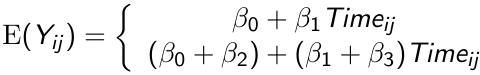

The top is control and bottom is treatment. By allowing an index for the j^th measurement we allow participants to have measurement in unequal time periods.

Consider the 3 hypotheses which could be tested:

H0: β₃ = 0 for testing parallelism between groups
H0: β₁ = 0 for testing flatness of change over time
H0: β₂ = 0 for testing differences between groups

Quadratic Trends

Higher order terms should be tested (and removed from the model if appropriate) before the lower order terms

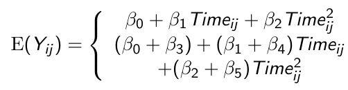
In the above we would first test β₂ = 0 and if this fails to be rejected we can remove the term and test β₁ = 0

To avoid potential problems with collinearity we center the variable of time around their mean before squaring it in order to include it as a quadratic term

Linear Splines

There are application in which the mean response cannot be modeled accurately using a polynomial, like when the mean response increases rapidly for some duration and then more slowly thereafter. In such a case a linear spline model would be appropriate.

Assume the mean response follows a linear trend, but the parameters change at a known time point t*; We can write the following linear spline model with a knot at time t*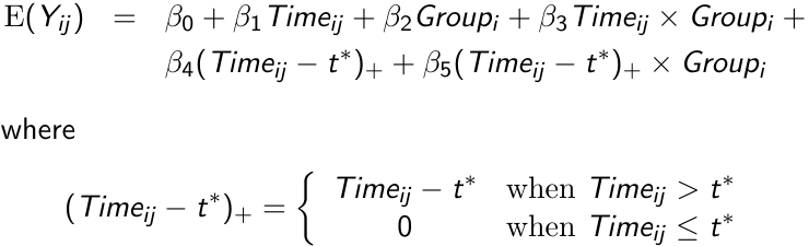

We can then write the model separately for each group before and after t*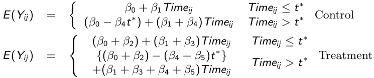

We can test the following hypotheses:

H0: β₃ = β₅= 0 for testing differences in patterns of change
H0: β₃ = 0 for testing group differences in patterns of change prior to t*
H0: β₄ = β₅= 0 for testing changes in the linear trend model after t*

Comparing Nested Models

When comparing nested models with respect to mean response, we can compute a likeliood ratio test (LTR) by running an ML (not REML) under the two models; full and reduced.

For example: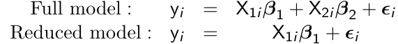

testing for β₂ = 0 is given by:
LTR = 2 (ℓ(β₁, β₂) - ℓ(β₂))

For non-nested models we can use AIC or BIC:
AIC = -2(ℓ - c)
BIC = -2(ℓ - log(n)*c)
Where ℓ is the maximized log-likelihood, c is the number of regression parameters and n is the number of subjects. Select the model that minimized AIC or BIC. The disadvantage of this method is they are empirically/evidence based and we cannot use them to perform any inference.