Linear Mixed Effects Modeling

The simplest mixed effect model is a random intercept model where Z_i = 1;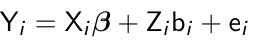

The random intercept model can be interpreted as the effect of all unobserved subject-specific variables (b_i) on the linear predictor.

Random slopes of time-varying covariates (δ) can be interpreted as interaction of unobserved subject specific covariates with observed time-varying covariates.

We can also include a random effect with a time-invariate covariate b_i (e.g. treatment group) to produce a heteroscediastic random intercept Z_i0 + Z_i1b_i.

Two-Stage Formulation

An alternative formulation of the mixed effects models is a two-stage formulation, in which we first specify a within subject or level-1 model where the occasion specific linear predictor is a function of time-varying covariates. Then a between subject or level 2 model is specified: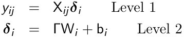

Some elements of δ_i are constant and some depend only on the observed covariates.

Consider the following with a random intercept and a random slope for time: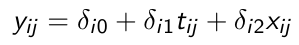

x_ij is a time-varying covariate and w_i is a time-invariant covariate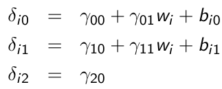

The redirected form is obtained by substituting the level-2 model into level-1 model. We then substitute level-2 into level-1 to produce the reduced form with a "cross-level interaction" term γ₁₁w_it_ij

• The two formulations are equivalent but it can have an impact on the types of models being considered
• The two-stage formulation encourages inclusion of many cross-level interactions and few same-level interactions
• Due to an abundance of interactions in the two-stage formulation, we usually center around the mean all variables except time. In our example, centering of w_i makes γ₁₀ interpretable as the mean effect of t_ij when t_ij when w_i takes it mean value.

Unobserved Confounders

In longitudinal studies, it is often said the "subjects serve as their own controls" when considering time-varying covariates. This seems to imply that all subject-level observed and unobserved covariates have been controlled for, but this is NOT true since this omitted covariates may correlate and hence be confounded with the time-varying variables of interest. If Cov(x_ij, u_ij) != 0, then we will have omitted variable bias; We say that x_ij is endogenous or correlated with the random intercept b_i0

Centering

Cov(x_ij, u_ij) = 0 if x_hat_i = x_hat_j for any i,j; We can then avoid omitted variable bias by subject-mean centering x_ij, forming the instrumental variable x_ij^d = x_ij - x_hat_i and running the following model: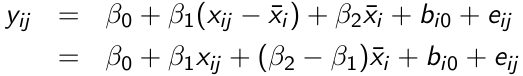

β₁ can be interpreted as a purely within-subject (or longitudinal) effect and β₂ as between-subject (or cross-sectional) effect. A test of the null hypothesis β₁ = β₂ is equivalent to the Durbin-Wu-Hausman test for exogeneity.

Linear Fixed Effects Models

Fixed effects linear models are formulated as: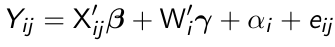

where X denotes a q*1 vector of time-varying covariates, Wi denotes a (p-q)*1 vector of time-invariant covariates and α_i are fixed effects representing the time-invariant unobserved confounders, and e_ij remains the random within-subject errors.