Module 9: Hypothesis Testing
The "effect" of a particular factor on some health outcome can be described as a parameter. Statistical hypothesis testing begins with a probability model assuming there is no effect or a null hypothesis (H0) and deciding whether there is sufficient evidence to reject the null hypothesis in favor of the alternative hypothesis (H1). Think of it like a legal trial; innocent until proven guilty.
One-sided Hypothesis: H0: θ = θ0 vs H1: θ > θ0 (or θ < θ0)
Two sided Hypothesis: H0: θ = θ0 vs H1: θ != θ0
We test H0 by finding an appropriate subset R ⊂ x, the rejection region. R is defined by R = {x : T(x) > c}; where T is a test statistic and c is a critical value.
- If X ∈ R -> reject null hypothesis
- If X !∈ R -> retain the null hypothesis
Errors
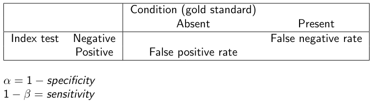
Type I error or false positive is rejecting H0 when it is true. α represents the probability of this error (typically set at .05)
Type II error or false negative is failing to reject the null when it is false. Probability represented by β.
Conducting and Interpreting the Test
- Define null and alternative hypothesis
- Set a desired α level. We choose a critical value such that: P(T(x) > c | θ = θ0) = α
- Collect data
- Calculate the observed test statistic value and compare to the critical value
- Make decision
P-value is the smallest critical value at which the test leads to rejecting the null hypothesis. It is a probability, when assuming the null is true, of obtaining a test statistic at least as large as the one we observed.
- p < α -> reject null
- p > α -> retain null
Retaining the hypothesis does not mean the null is true, it is interpreted as a lack of evidence to accept the alternative.
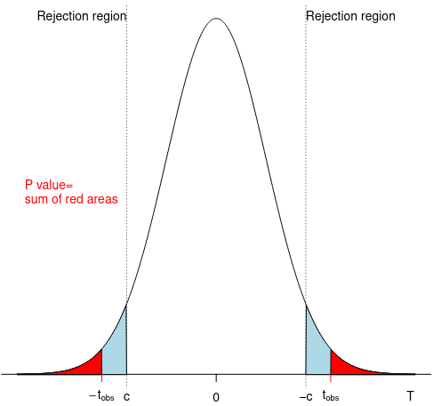
We expect the data to come from the center of the distribution, there is a lower probability of pulling data from tails. If our sample statistic occurs at the tail, then this may not be a representative distribution.