Survival Analysis II

In survival data the dependent variable is always survival time (or time until an event with the potential to censor observations). The independent variable can be any type; Continuous, ordinal or categorical. We assume the observations are independently and randomly drawn from the population.

Kaplan-Meier estimator allows crude comparison between two groups, but it does not provide an effect estimate or allow adjustment for covariates.

Cox Proportional Hazards Model

In 1972 Sir David Cox introduced a survival model in which the hazard function changes with time only through the baseline function.

We can model the hazard as a function of the exposure and quantify the relative hazard, which allows for adjustment of covariates. This is the instantaneous failure rate, or the event rate over a small interval or time. The hazard ratio does not depend on time. The hazard baseline function is modeled as: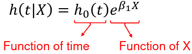

A hazard ratio at time t for a change in X: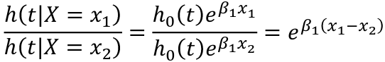

The baseline hazard function, h₀(t) when X=0, is treated as a nuisance function and is left unspecified (non-parametric part of the model). The covariates affect the hazard function multiplicatively through the function exp(Beta*X) (the parametric part of the model).

The model is therefore called a semi-parametric model. It is suitable when we are more interested in the parameter estimates (effects of covariates) than the shape of the hazard. Fit by maximizing the partial likelihood.

X = 0

X = 1

Hazard ratio X=1 vs X=0

CI is similar to logistic regression, we only model the hazard rather than the odds. Situations in which you might expect the logistic and PH regression results to differ:

Common event (cumulative risk for the event is not small)
Differential loss to follow-up (loss differs by exposure)
Exposures change over follow-up

Tied Event Times

Breslow's Method
- An approximation to the exact adjustment
- Default option in SAS
Efron's method
- A different approximation to the exact adjustment
- A better approximation than Breslow's method
- Default in R / SAS: "ties=efron" in PROC PHREG
Kalbfleisch and Prentice's "exact" method
- Assumes ties are due to imprecise measurement of time
- Most computationally-intensive method (all possible ordering of tied data is considered)
- Not available in R / SAS: "ties=exact" in PROC PHREG

All will give the identical estimates if there are no ties.

Proportional Hazards Assumption

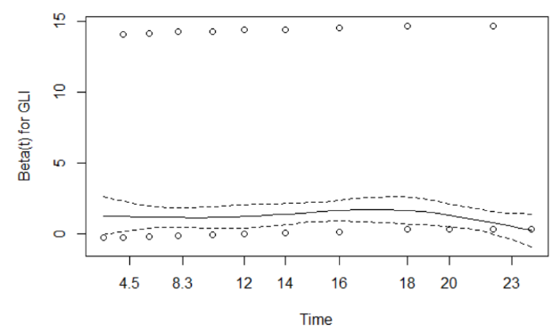
Beta should not change with time if the proportional hazards assumption holds.

H₀: Proportional hazard is satisfied
Conclusion: We fail to reject the null hypothesis, so no evidence of departure from the PH assumption

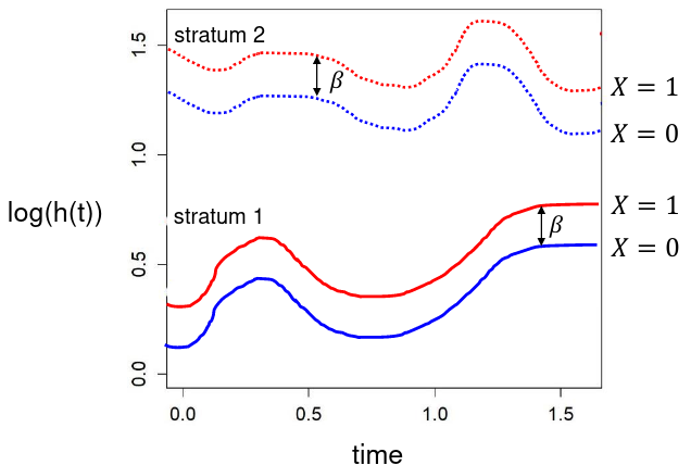
Graphical Method: log(-log(S(t))) plot
- The natural logs of h(t | X) plotted against time are parallel for varying values of X, separated by Beta
- Likewise, the log of the negative log of S(t | X) plotted against time (or log(time)) are parallel for varying values of X, separated by Beta
Schoenfeld Residuals
- Suppose subject i has an event at time t_t
- The Schoenfeld residual for subject i and covariate X is:
  - x_i- x_bar(t_i), where x_bar(t_i) is the estimated mean of X based on the subjects at risk at time t_i(similar to observed - expected)
- A test of the PH assumption is based on a test of the correlation between sccaled Schoenfeld residuals and a function of time
  - If the PH assumption is satisifed the Schoenfeld residuals should be uncorrelated with time
  - A significant test (small p-value) suggests that the PH assumption fails
- If the proportional hazards assumption is satisfied the plot should look like a horizontal line
- In R: 'cox.zph(linreg)'
Time-varying Effects
- SAS and R have internal algorithms to build the "time-varying covariates", this is NOT the same as including a time covariate interaction in the model.
- In this method we think of Beta as a function of time:
  Beta = a + bt
Martingale Residuals (SAS Only)
- Using ASSESS statement in SAS
- Assess both functional form and proportional hazards assumption for each covariate using simulation
- A set value needs to be set to reproduce results
- The observed path (solid line) should not be extreme compared to the simulated paths (dashed lines)

Which Test to Use?

A method should be choosen ahead of time. Tests based on Schoenfeld residuals and time-varying effects are the most commonly reported.

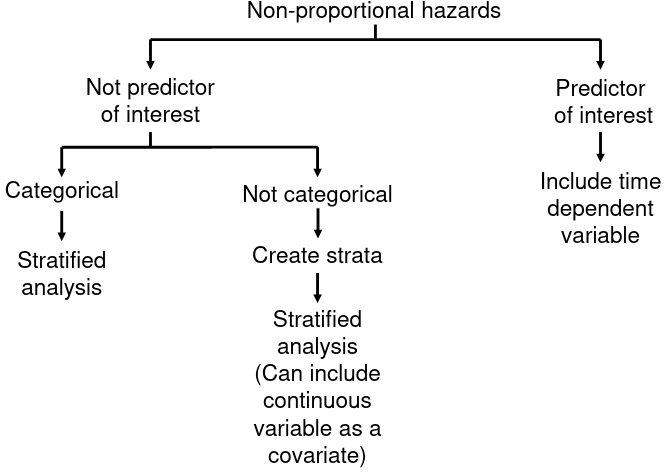
Non-Proportional Hazards

If the variables failing PH assumption are not of interest we can use a stratified PH model in which a different baseline hazard is fitted per stratum.

If the variables failing PH assumption are of interest include the time-dependent variable and deal with complicated conclusion of HR varying over time. This can be hard to interpret.

Defining Strata

Each stratum use a separate baseline hazard: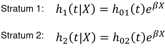

The Beta is the same for each stratum and the effect of the variable is now part of the baseline hazard.

For example, if we create stratum based on sex, we can no longer use the model to compare hazards across sex, as the effect of sex is now part of the baseline hazard, which we do not estimate.

We compare the exposed subjects to unexposed subjects within the same stratum. We cannot compare exposed subjects to unexposed subjects across different strata.

Stratifying Continuous Variables

Create a categorical variable defining strata based on the continuous variable
Use this categorical variable to stratify the analysis
Include the continuous variable as a covariate in the model to account for residual association within the strata. Results are difficult to interpret

You can keep an interaction between X and time in your model if it failed the PH assumption, but you cannot interpret the parameter estimate since it is a function of time.

Time-Dependent Exposures

Some exposures vary over time, and this varying exposure is important to assess. The Cox model can be extended to accommodate this. For example, someone who has been smoking since they were young has different survival rate compared to someone who just started smoking.

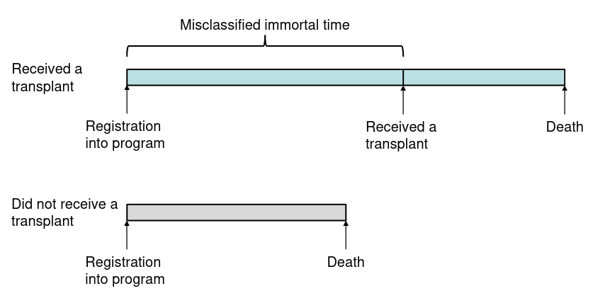
Immortal Time Bias - Effect of an exposure can be biased toward survival if there is a delay between entry into study and exposure.

R Code

library(survival)
framdat4 <- read.csv("framdat4.csv", header=T, na.strings=c("."))

## Cox Proportional Hazards regression
### Crude Model    

# Fit the model: coxph()
fit.1 <- coxph(Surv(chdtime, chd_sw) ~ GLI, data=framdat4)
summary(fit.1)


### Adjusted Model
fit.2 <- coxph(Surv(chdtime, chd_sw) ~ GLI+AGE+SPF+CSM+FVC+MRW, data=framdat4)
summary(fit.2)

## Assess the PH assumption
### Log(-Log(Survival)) Plot
fit.km <- survfit(Surv(chdtime, chd_sw) ~ GLI, data=framdat4)

# Method 1: use the fun="cloglog" option
plot(fit.km, col=c("black", "red"), fun="cloglog",  main="Log of Negative Log of Estimated Survival", 
     xlab="time", ylab="log(-log(survival))", cex.main=1.5, cex.axis=1.5, cex.lab=1.5)
legend(x=12, y=-3.5, legend=c("No GLI","GLI"), col=c(1,2), lwd=1, cex=1.2)

# Method 2: calculate the logs manually
plot(log(fit.km$time),log(-log(fit.km$surv)), main="Log of Negative Log of Estimated Survival", 
     xlab="log(time)", ylab="log(-log(survival))", cex.main=1.5, cex.axis=1.5, cex.lab=1.5)
lines(log(fit.km$time[1:12]), log(-log(fit.km$surv[1:12])), lwd=2)
lines(log(fit.km$time[13:24]), log(-log(fit.km$surv[13:24])), lwd=2, col=2)
legend(x=2.5, y=-3.5, legend=c("No GLI","GLI"), col=c(1,2), lwd=2, cex=1.2)

### Schoenfeld residuals
# Assess the PH assumption: cox.zph()
test.1 <- cox.zph(fit.1)
print(test.1)
plot(test.1)

test.2 <- cox.zph(fit.2)
print(test.2)
plot(test.2)

### Time-Varying Covariates to assess PH assumption
# Use the 'tt' option
# (1) Interaction with time
fit.a <- coxph(Surv(chdtime, chd_sw) ~ GLI+tt(GLI), data=framdat4, 
                   tt=function(x,t,...)x*t)
summary(fit.a)
# plot HR
plot(c(0:25), exp(1.46-0.024*c(0:25)), type="l", xlab="Time (years)", ylab="HR", col="blue", lwd=2)

# (2) Interaction with log(time)
fit.b <- coxph(Surv(chdtime, chd_sw) ~ GLI+tt(GLI), data=framdat4, 
                   tt=function(x,t,...)x*log(t))

summary(fit.b)
# plot HR
plot(c(0:25), exp(1.28-0.05*log(c(0:25))), type="l", xlab="Time (years)", ylab="HR", col="blue", lwd=2)
 
### Stratified analysis
# Create age strata
age.group <- rep(1, nrow(framdat4))
age.group[ which(framdat4$AGE >44 & framdat4$AGE <55)] <-2
age.group[ which(framdat4$AGE >54 & framdat4$AGE <65)] <-3
age.group[ which(framdat4$AGE >64 & framdat4$AGE <75)] <-4

# Fit stratified model using strata() option
fit.s <- coxph(Surv(chdtime, chd_sw) ~ GLI+SPF+CSM+FVC+MRW+AGE+strata(age.group),
               data=framdat4)
summary(fit.s)

cox.zph(fit.s)

Revision #12
Created 7 November 2022 14:49:45 by Elkip
Updated 7 November 2022 17:35:42 by Elkip