Statistical Modeling
Statistical association analysis is not all about significance. There is much to consider when deciding covariates and choosing a model to represent the relationship.
Regression Modeling
- If we have a small number of variables we can manual assess confounding and collinearity by comparing models with each potential confounder.
- First we need to ask what a "small" number of variables; a number that is manageable for manual assessment of variable significance and confounding.
- If we have > 10 variables and need to cut variables
- Base on prior assumptions about confounders
- Base on a threshold p-value (maybe .2) from univariable analyses
- There's no test for confounding: 10% is not a hard rule, we might consider > 10% to be conservative
- When we have a large number of variables it becomes impossible to run manually, so we choose a systemic model to cut variables and reduce the model
- Beware of dropping important confounders or relying solely on measures such as AIC
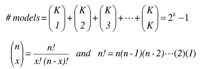
- If there are K variables (in an additive model without interaction):

Troubleshooting Regression Modeling
- Getting errors or weird results in a categorical variable with multiple categories
- Likely due to a small number of samples in some categories
- Fix: Combine categories in a way that makes sense to increase sample size in one group
- If the variable cannot be defined differently, consider excluding the variable initially and including it later on when we have less variables
- Sometimes we want to "force" a variable into a model, regardless of its significance or confounding
- This might occur when its something the readers want to know (age, sex, etc) or its the main exposure of interest
Variable Selection Methods
When no interaction exists, we have 3 primary approaches to variable selection:
- Forward
- Pick the variable most highly associated with the outcome
- Given that the variable is in the model, now pick from the remaining variables
- Continue until there are no more significant variables or all variables are in the model
- Stepwise Regression
- It is the same as the forward procedure except that at each step it looks at all variables in the model to see if they are still significantly significant (if not the variable is dropped)
- Pro:
- Speeds up process of searching through models
- More feasible than manual selection
- Cons:
- Blind analysis without thinking
- Backward methods
- Start with fully adjusted model
- Remove all variables starting with largest p-value
- Check for any confounding impact by comparing ORs before and after removal
- Stop when all remaining variables are significant or confound other variables
- Pro:
- Useful with small numbers of variables
- Cons:
- In practice it is impossible to use with a very large number of variables
Modeling with Interaction
Interaction is regarded as deviation from no interaction model, AKA multiplicative. In a multiplicative model, the order of the interaction terms can make a difference. In a hierarchical model lower order terms always come before higher order terms.
- Proceed backwards: Evaluate interaction then main effects.
- This may not be possible when possible parameters (2^k - 1) exceeds the sample size
- This can be hard to interpret and has little power for high levels of interaction.
- This procedure is applicable when there is a risk factor of interest and confounders
- Force all main effects into the model; perform stepwise regression analysis on the 2-way interactions
- It may be smart to only consider interactions having to do with the exposure of interest
- Be sure to have a hierarchical model
- Retain whatever 2-way interactions remained after step 1, perform a stepwise regression analysis on the main effects which are not part of the 2-way interactions retained
Model Selection
One can look at changes in the deviance (-2 log likelihood change)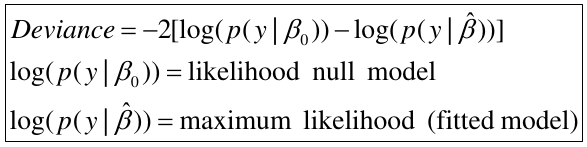
- Deviance = Residual Sum of Squares with normal data
- Problem - deviances alone do not penalize "model complexity", hence LRT is needed but only applied to nested models
- More common measures:
- AIC: Akaike's Information Criterion
- BIC, SC, SBC: Schawrtz's Bayesian Information Criterion
AIC & BIC
Both are based on likelihood. An advantage is you do not need hierarchical models to compare the AIC or BIC between models unlike -2 ln LR, the disadvantage is that there is no test or p-value that goes with comparison of models. A model with smaller values of AIC or BIC provides a better fit. When n > 7 the BIC is more conservative.
AIC and BIC can also compare non-nested models (a model where the set of independent variables in one model is not a subset of the independent variables in the other model).
The data must be the same.
Common Issues with Model Building
Collinearity occurs when independent variables in a regression model are highly correlated, or a variable can be expressed as a linear combination of other variables.
Problem: the estimate of standard errors may be inflated or deflated, so that the significance testing of the parameters becomes unreliable.
One strategy that should be used is to examine the correlations among potential independent variables, and give collinearity diagnostics. When two variables are collinear, drop one or create a new variable of both.
Risk Prediction & Model Performance
Calibration is meant to quantify how close predictions are to actual outcomes (goodness of fit)
Discrimination refers to the ability of the model to distinguish correctly the two classes of outcome
This is generally only used for dichotomous outcomes.
A model that assigns a probability of 1 to all events and 0 to nonevents would have perfect calibration and discrimination. A probability of .51 to events and .49 to nonevents would have perfect discrimination and poor calibration.
Calibration Metrics
Calibration at large: how close is the proportion of events to the mean of predicted probabilities.
Home-Lemshow Decile Approach (Logistic Regression)
- Divide the model-based predicted probabilities of size n_j
- In each decile calculate the mean of predicted probabilities p_bar_j and comare it to the observed proportion of events in that decile (r_j):

- Degrees of freedom equal to number of groups minus 2
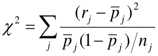
Sensitive to small event probabilities in categories - a construct of adding 1/n_j to p_bar_j in the denominator. It is sensitive to large sample sizes.
This solution actually has serious problems; results can depend markedly on the number of groups and there's no theory to guide the choice of that number. It cannot be used to compare models.
ROC (Receiver Operating Curve)
Plots sensitivity (true positive) for different decisions and look for the best trade off between sensitivity and specificity (true negative).
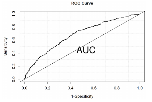
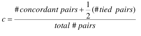
- The area under the curve (AUC) is a summary measure called the c statistic;
- c is the probability that a randomly chosen subject with the event will have higher predicted probability of the event than a randomly chosen subject without the event (a measure of discrimination)
- All pairs of subjects with different outcomes are formed
- Pairs where the subject with the higher predicted value also has the higher outcome are concordant, vice versa is discordant
- > .8 is very good and < .6 is useless
Prediction, Goodness of Fit
This value can be interpreted as the "true" predictive accuracy. Methods to validate:
- Randomly split the samples into training and tesing
- Cross-validation - divide samples into k sub-samples and test on 1/k groups
- Boostrap - resample with replacement for a new sample
With any of these the analysis should be repeated many (over 100) times.
Harrell's c Survival Analysis
Calibration at large - compare how close the mean of model-based predicted probabilities at time t is to the Kaplan-Meier estimate at time t
Calibration by decile - replace rates/proportions in deciles with their Kaplan-Leier equivalents; change df to 9
- Call any two subjects comparable if we can tell which one survived longer
- Call two subjects concordant if they are comparable and their predicted prbabilities of survival agree with their observed survival times
- 'c' defined as probability of concordance given comparability
Multiple Comparisons
The significance is the probability that, in one test, a parameter is called significant when it is not (Type I error)
Multiple comparisons asks what the overall significance is when we test several hypotheses.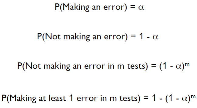
We can apply the Bonferroni correction (.05/n) to account for multiple comparisons.
False discovery rate - False positives among the set of rejected hypotheses, often used in studying gene expression.