Missing Data

Missing data is common in epidemiology studies, and always observed in longitudinal studies. Inadequate handling of missing data may cause bias or lead to inefficient analyses. If an estimate is incomplete, we can remove it without introduce bias. If a variable is heavily missing, it may be appropriate to remove the variable then remove all incomplete records.

There is a difference between missing and "unknown" data. Ex. someone refusing to report income on a survey would be considered missing, but an individual who has no preference between republican and democrat candidates may be considered a new category of "do not know".

Missing Data Mechanisms

The way to analyze incomplete data depends on the underlying missing data mechanisms. Ex. Is the missing data the same between males and females? Are values which are higher or lower more likely to be missing?

Missing completely at random (MCAR): No systematic differences between the missing values and the observed values.
- Ex. Blood pressure measurements missing because of a broken tool
- In this case, the missing data mechanism is ignoreable, and missing data for the outcome can be ignored
Missing at random (MAR): Any systemic difference between the missing values and the observed values can be explained by differences in observed data.
- Ex. Missing blood pressure measurements may be lower than those measured because younger people are more likely to be missing measurements.
Missing not at random (MNAR): Even after the observed data are taken into account, systematic differences remain between the missing values and the observed values.
- Ex. people with hypertension missing clinic appointment because of headaches

MAR vs MCAR

If the data are MCAR we can analyze complete cases
If the data are MAR missing data should not be ignored
Deterministic imputation can introduce bias/overconfidence, particularly when more than 10% of the data is missing
- Marginal imputation reduces power and bias results toward the null
We can distinguish MCAR from MAR by observing the distribution of the indicator variable and see whether it is correlated with the observed data

Missing Data Patterns (Univariate)

Suppose we have a sample of size n, with some missing data points where: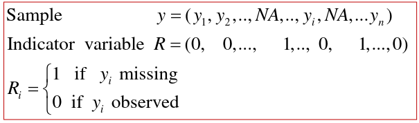

The pattern of missing data can be described via the distribution of the indicator variable R: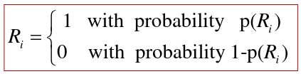

If the probability that R_i = 1 is independent of the value y_i, for any index i, the missing data pattern is ignorable. Equivalently. data are MAR
- The observed data are a random sample of complete but unobserved sample
- We can remove the data with the only effect being a decrease in power due to sample size
If the probability that R_i = 1 is NOT independent of the value y_i, for any index i, the missing data pattern is NOT ignorable, i.e. MNAR, the data are informatively missing
- The observed data does not represent a random sample of complete data.
- Missing data is not ignorable, removing it may introduce bias

Missing Data Patterns (Mutlivariate)

Assume we have a multivariate dataset with outcome Y and covariates X₁-X_k

Suppose we only have missing data on Y. As in the univarite case, the patterns of missing data can be described via the distribution of the indicator variable R.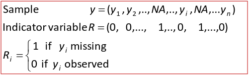

Where R_i = 1 has probability p*R_i, and R_i = 0 has probability 1-p*R_i

If the probability that R_i = 1 is independent of the value y_i, and the covariates for any index, the missing data mechanism is ignorable and the data are MCAR.
If the probability that R_i = 1 is independent of the value y_i, but is depedent the covariates for any index, the missing data mechanism is ignorable and the data are MAR. However, the observed sample may not be a random subsample of the complete one.
If the probability that R_i = 1 is dependent of the value y_i, the missing data pattern is NOT ignorable, i.e. MNAR, the data are informatively missing

Imputation

Imputation is the idea that we can fill in the missing data using either a deterministic or stochastic method or combination of both.

Deterministic imputation
- Refers to the situation given specific values of other fields, when only one value of a field will cause the record to satisfy all of the edits, such as using the mean or median
Stochastic (regression) imputation
- This method uses regression, it adds a random error term to the predicted value and is therefore able to reproduce the correlation of X and Y more appropriately.

Other procedures include EM algorithm, Markov Chain Monte Carlo Bayesian method, weighted methods (IPW), etc.

Multiple Imputation

To avoid the bias of the deterministic imputation, the following methods are applied:

Imputing the missing data randomly
Repeating the imputation many times
Analyzing each imputed data set
Summarizing the estimate by mean over the different sets and correct the variance

There is a paper on this by Sterne et al which explains the pitfalls and reporting procedure, but I will not go into detail here.

Other methods to fill-in missing data

Marginal mean imputation: replace the missing y-values with the marginal mean based on the complete cases.
- This biases the data toward the null hypothesis, if the data are MCAR
Conditional mean imputation: replace the missing y-value with the conditional mean (E(Y | X))
- This imputation biases the data toward the hypothesis of an association with the covariates

Note that to assess confounding we compute crude estimates against adjusted with the same imputed data. It is very important to use the same dataset to keep results consistent.

R Code

framdat2 <- read.table("C:/Users/liuc/Documents/BS852/BS852_Fall2021/class12/framdat2.txt",header=T, na.strings=c("."))
summary(framdat2)

# Proportion missing per variable
for(i in 1:ncol(framdat2)){
  print(names(framdat2)[i])
  print(sum(is.na(framdat2[,i]))/nrow(framdat2))
} # 6 of the variables have missing data

# Distribution of incomplete cases
num.miss <- apply(is.na(framdat2),1,sum)
table(num.miss) 
length(num.miss[which(num.miss %in% c(1:6))])

MRW <- is.na(framdat2$MRW)

# Missing MRW
table(MRW)
# Missing GLI by sex
table(framdat2$SEX, MRW)/apply(table(framdat2$SEX, MRW),1,sum)

# Is missing GLI associated with sex?
summary(glm(MRW~framdat2$SEX, family=binomial(link = "logit")))

cbind(framdat2$FVC, is.na(framdat2$FVC))[1:28,]

sim.data <- read.csv("C:/Users/liuc/Documents/BS852/BS852_Fall2021/class12/sim.data.csv",header=T, na.strings=c("."))

# crude and adjusted models
summary(lm(y ~ SMOK, data=sim.data))

summary(lm(y ~ SMOK + Age + BMI + SEX, data=sim.data))

# 10% MCAR
set.seed(1234)
R <- rbinom(nrow(sim.data), p=0.10, size=1) # randomly select data to keep

mod.10mcar.crude <- lm(y ~ SMOK, data=sim.data[R==0,])

mod.10mcar.adj <- lm(y ~ SMOK + Age + BMI + SEX, data=sim.data[R==0,])

summary(mod.10mcar.crude); summary(mod.10mcar.adj)

# Marginal Mean Imputation
# 10% MCAR
set.seed(1234)
R <- rbinom(nrow(sim.data), p=0.10, size=1)

mean.obs.y <- mean(sim.data[R==0,]$y) ## complete data
sim.data$y.imputed <- sim.data$y 
sim.data$y.imputed[R==1] <- mean.obs.y
boxplot(list(raw=sim.data$y, imputed=sim.data$y.imputed))
 
mod.imputed.crude <- lm(y.imputed ~ SMOK, data=sim.data)
summary(mod.imputed.crude)

mod.imputed.adj <- lm(y.imputed ~ SMOK+Age+BMI+SEX, data=sim.data)
summary(mod.imputed.adj)

# Conditional Mean Imputation
# 10% MCAR
set.seed(1234)
R <- rbinom(nrow(sim.data), p=0.10, size=1)

imp.model <- lm(y ~ SMOK+Age+BMI+SEX, data=sim.data[R==0,])
summary(imp.model)
imp.model$coeff
sim.data$y.imputed[R==1] <- imp.model$coeff[1]+
                                imp.model$coeff[2]*sim.data$SMOK[R==1]+
                                imp.model$coeff[3]*sim.data$Age[R==1]+
                                imp.model$coeff[4]*sim.data$BMI[R==1]+
                                imp.model$coeff[5]*sim.data$SEX[R==1]
boxplot(list(raw=sim.data$y,imputed=sim.data$y.imputed))
 
mod.imputed.crude <- lm(y.imputed ~ SMOK, data=sim.data);  summary(mod.imputed.crude)

mod.imputed.adj <- lm(y.imputed ~SMOK+Age+BMI+SEX, data=sim.data); summary(mod.imputed.adj)

# Distinguish MCAR from MAR
set.seed(1234)

p.miss <- c()
for (i in 1:nrow(sim.data)){
  p.miss[i] <- max(0, sim.data$Age[i]/400 + runif(n=1, min=0, max=0.02))
}

R <- c()
for (i in 1:nrow(sim.data)){
  R[i] <- rbinom(n=1, size=1, p=p.miss[i])
}

mod.mar <- glm(R ~ sim.data$Age+sim.data$BMI, family=binomial)
mod.step <- step( mod.mar, scope = R~.) 
summary(mod.step)


hdl.data <- read.csv("hdl_data.csv",header=T, na.strings=c("."))

hdl.data.2 <- hdl.data[, c("SEX","BMI5","AGE5","ALC5","CHOL5","TOTFAT_C")]
summary(hdl.data.2)

summary(lm(TOTFAT_C~SEX+BMI5+AGE5+ALC5+CHOL5, data=hdl.data.2))

# Create missing data indicator for TOTFAT_C
R <- rep(0, nrow(hdl.data.2))
R[which(is.na(hdl.data.2$TOTFAT_C)==T)] <- 1

mod.mar <- glm(R ~ AGE5 + BMI5 + SEX, family = binomial, data=hdl.data.2)
step(mod.mar, scope=R~.)

library(Amelia)

set.seed(1234)
imp.data <- amelia(hdl.data.2, m=10)  ## 10 imputed datasets
summary(imp.data[[1]][[1]])

beta.bmi <- c(); se.beta <- c()
for(i in 1:10){
  mod <- lm(TOTFAT_C~SEX+BMI5+AGE5+ALC5+CHOL5, data=imp.data[[1]][[i]])
  beta.bmi <- c(beta.bmi,   
  summary(mod)$coefficients[grep("BMI5", row.names(summary(mod)$coefficients)),1])
  se.beta <- c(se.beta, 
  summary(mod)$coefficients[grep("BMI5", row.names(summary(mod)$coefficients)),2])}
   
beta.mean <- mean(beta.bmi); beta.mean
beta.var <- mean(se.beta^2) + var(beta.bmi)
beta.mean/sqrt(beta.var)

# significance based on Wald test
2*(1-pnorm(beta.mean, 0, sqrt(beta.var)))

beta.bmi <- c(); se.beta <- c()
for(i in 1:10){
    mod <- lm(TOTFAT_C~ BMI5, data=imp.data[[1]][[i]])
    beta.bmi <- c(beta.bmi, 
        summary(mod)$coefficients[grep("BMI5", row.names(summary(mod)$coefficients)),1])
    se.beta <- c(se.beta, 
        summary(mod)$coefficients[grep("BMI5", row.names(summary(mod)$coefficients)),2])}

beta.mean <- mean(beta.bmi); beta.mean
beta.var <- mean(se.beta^2) + var(beta.bmi)
beta.mean/sqrt(beta.var)

# # significance based on Wald test
2*(1-pnorm(beta.mean, 0, sqrt(beta.var)))

Revision #4
Created 12 December 2022 15:04:20 by Elkip
Updated 12 December 2022 16:18:33 by Elkip