Statistical Methods in Epidemiology
BS852: Statistical methods for interpreting statistical analysis and addressing confounding or interaction in observational studies
- Analysis of 2x2 Tables
- Stratification and Interaction
- Standardization
- Matching
- Logistic Regression
- Logistic Regression in Matched Studies
- Survival Analysis I
- Survival Analysis II
- Model Fit & Concepts of Interaction
- Poisson Regression
- Statistical Modeling
- Missing Data
Analysis of 2x2 Tables
Review of Measures of Association
| Exposed |
Unexposed |
||
| Disease |
a |
b |
m1 |
| No Disease |
c |
d |
m0 |
| n1 |
n0 |
n |
m1, m0, n1, and n0 are marginal totals and n is the overall total
Prevalence is the proportion of sampled individuals that possess a condition of interest at a given point in time.
Incidence is the proportion of individuals that develop a condition of interest of interest of a period of time.
The Odds Ratio (OR) of an outcome are the ratio of the probabilty that the outcome occurs to the probability that the outcome does not occur:
OR = ((a / n1) / (c / n1)) / ((b/n0) / (d/n0)) = (a/c) / (b/d) = ad / bc
Risk Ratio (RR), or relative risk, compares the risk of a health event among one group with the risk among another group:
RR = (a / (a + c)) / (b / (b + d)) = (a / n1) / (b /n0)
We would interpret the RR as: People in "group A" have RR times the risk for being a case compared to the people in "group B".
The OR is always farther from 1 than RR (unless both equal 1). If a rare disease OR ~= RR
Risk Difference (RD):
RD = a / (a + c) - b / (b + d)
RR and RD are only appropriate for incidence or prevalence studies, NOT case-control studies.
When testing if there is an association between two variables (H0 = Slope is 0), we could also set RR = OR = 1 or RD = 0.
Common Tests For Association
- Standard Chi-Square statistic (also called Pearson chi-square)
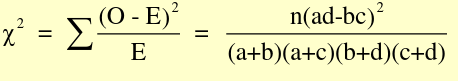
Where O is observed and E is expected, with 1 degree of freedom (n-1)
- Mantel-Haenszel Chi-Sqaure statistic
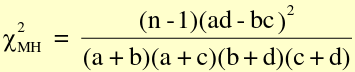
Similar to standard chi-square, with n-1 instead of n
- Large sample Z statistic to compare proportions
- Large sample Z statistic for exposed events
For a 2x2 Table:
- The standard chi-square and Mentel-Henszel chi-square statistic are completely equivalent to each other
- The large sample z for proportions and exposed events are completely equivalent to each other
- The z statistics and chi-square statistics are nearly equivalent to the first two
- The z statistics can be looked up via R or textbook appendix
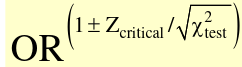
Confidence Intervals
CI is not a probability! Proper interpretation of a 95% CI: If we repeatedly take samples of the same sample size from the population and build 95% confidence intervals for the OR, then we are 95% confident that the interval covers the true OR.
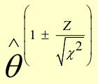
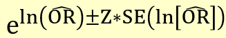
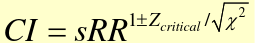
A test-based CI for OR:
Confounding in Epidemiology
Bias refers to any systematic error in an epidemiological study that results in an incorrect estimate of the true effect of an exposure on an outcome of interest.
Confounding occurs when a variable influences both the dependent (outcome) and independent (exposure) variable, causing a spurious association. When confounding is present a measure of association may change substantively in comparing the measure without adjustment.
If a measure, such as RR or OR, changes by more than 10% we conclude there is confounding.
Confounder, Mediator, and Collider:
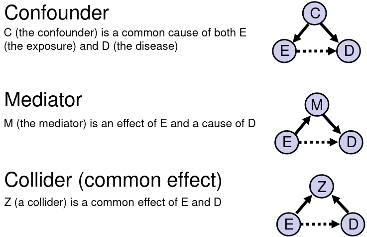
If we are interested in the total effect of an exposure on an outcome we should adjust for confounders, but not colliders or mediators. If the confounder is a categorical variable, we may stratify the samples on the confounder.
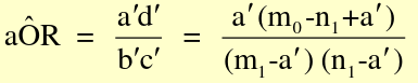
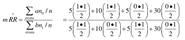
Mantel-Haenszel Method
The Mantel-Haenszel Method (mOR) is a weighted average of the OR for each stratum:
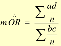
(bc)/n is the weight for each stratum.
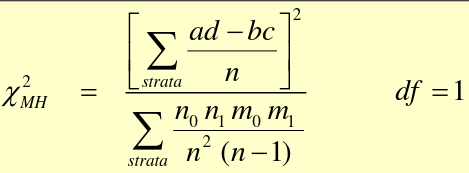
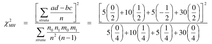
We hypothesis test with the MH Chi-square test for summary measure:
H0: OR1 = OR2 = OR3.... = 1 or mOR = 1
Ha: OR1 = OR2 = OR3.... != 1 or mOR != 1
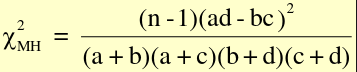
For testing a single 2x2 table with the MH Chi-Square Test for a summary measure:
For analysis of several 2x2 tables:
A Flow-Chart: Steps to Follow
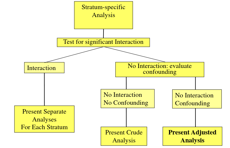
Stratification and Interaction
Which Summary Measure to Use?
- Weighted averages are usually best
- Mantel-Haenszel is easy to compute and can handle zeros
- MLE measures are difficult and typically require a computer
Weighted Average in MH Summaries
Consider the following table:
| Sample 1 |
Sample 2 |
|
| n |
30 |
70 |
| x_bar |
5 |
8 |
Weighted average of population -> ((30*5)+(70*8))/(30+70) = 7.1
The average mean is closer to the cohort with a larger sample size. We can calculate any weighted average with the general form:
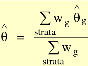
Where theta_hat is an estimator, such as mean or OR.
The MH Odds Ratio and RR can be described as weighted averages:
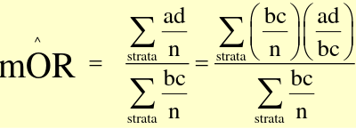
Where the weights are (b*c)/n
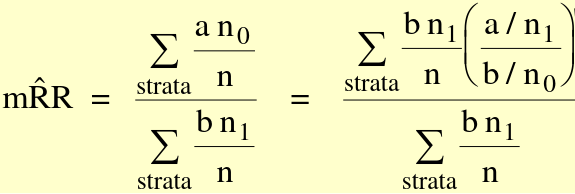
Where (a/n_1) / (b/n_0) is the risk ratio in each stratum, (b*n_1 / n) is the weight
Assumptions of Mantel-Haenszel Summary Measures
- Observations are independent from each other
- All observations are identically distributed
- The common effect assumption should hold:
- Follow-up cohort study - The stratum-specific risk ratios are all equal across the strata
- Case-control - The stratum specific odds ratios are all equal across the strata
MH measures are biased if the correctness of the common effect assumptions cannot be justified.
An extreme example: When interaction exists with protective and detrimental effects across strata; Protective effects negative in numerator in a stratum, and detrimental effects positive in numerator in another stratum.
Precision-based Summary Estimators
Also called Woolf's Method. Precision-based summary estimators are also weighted averages. Weighing each stratum according to its sampling error gives the most weight to the strata with the smallest variance. Precision-based are designed to have the greatest precision (smallest standard error). For Ratios we often take the log scale for a more symmetrical distribution. The general approach:
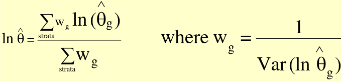
This is the sum of the products of each stratum-specific ratio times its weight, all divided by the sum of weights.
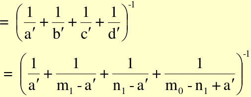
Precision-based Summary Odds Ratio
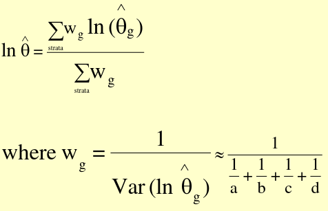
Thus, Var(ln(OR_hat) ~ 1/a + 1/b + 1/c + 1/d
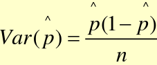
Precision-based Summary Risk Ratio
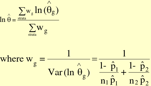
Thus the Var(ln(RR_hat)) = ((1-p_hat1)/(n_1*p_hat1) + (1 - p_hat2)/(n_2*p_hat2))
Confidence Intervals of Summary Measures
There are 2 types of CI intervals: Test-based (from a test statistic) and Precision-based (uses standard error). Most of the time both will yield very similar intervals.
Test-Based CI
Precision-based CI
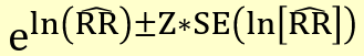
Where the standard error is the square root of the variance above.
Comparision
Precision-based summary ratios are straightforward, and best when the number of strata is small, and sample size within each strata is large. Cannot be calculated when any cell in any stratum is 0 as log(0) is undefined, though one could correct .5 at risk of bias.
MH Method can handle 0 cells. The assumption is that all counts are large enough, if there are small counts in some strata the CI will not be valid.
Hypothesis Testing of Interaction
Tests for interaction (effect modification):
H0: OR1 = OR2 = ... = ORg / H0: RR1 = RR2 = ... RRg
Tests of Association from Stratified 2x2 Tables:
H0: No association and the summary (adjusted) measure = 1
Breslow-Day Test
This is default test for interaction in SAS.
Steps: Calculate summary OR, use summary OR to get expected number of exposed cases per strata, if no interaction compare with actual number of exposed cases for each strata
H0: OR1 = ... ORg (g strata)
H1: at least two measures are different
Conclusion: We have [in]sufficent evidence to [reject/accept] the null hypothesis that all the associations between X and Y adjusted by strata are equivalent.
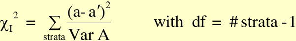
Where a = observed value in gth stratum and a| = fitted or expected value of under H0 in gth stratum
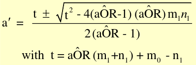
a| should be comparable with table margins (determines whether to add or subtract the radical)
Variance under H0 in the gth stratum:
Assume a common OR (mOR) and create adjusted:
Woolf Test
- Can be used for RR or OR
- Calculate summary OR, compare strata-specific ORs to summary OR
- .5 is added to each cell as a small-sample adjustment (optional)
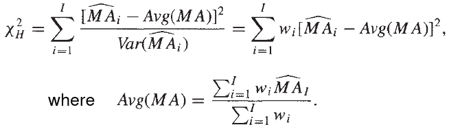
Most often, Breslow-Day and Woolf's test produce similar test statistics. Woolf's method has a theoretical derivation of the weights based on large counts in each cell. If there are small counts in a strata, the CI is invalid.
Standardization
The objective of standardization is the compare the rates of a disease (or outcome) between population which differ in underlying characteristics (age, sex, race, etc) that may affect the overall rate of disease; In essence it's another way to account for confounding.
Standardization of Rates
The difference between crude rates and standardized rates is that the crude rates are calculated on the population under study, whereas standardized rates are based on particular characteristic(s) as standard. If the rates are calculated based on the specific characteristic(s), they are called specific rates (eg. age specific mortality rates, or sex specific mortality rates).
While the MH and Precision based tests assume uniformity of estimates across strata, standardized estimators do not. Thus, these summary measures ignore non-uniformity and mask interactions.
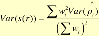
CI of Standardized Rate
Variance:
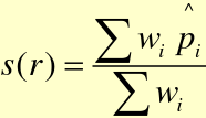
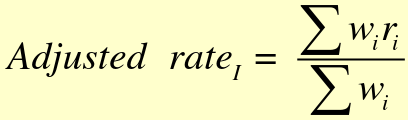
Standardized Rate is a Weighted Average:
Variance for a Standardized Rate:
There are two approaches to Standardization of Rates:
Direct Standardization (Most Common)
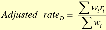
wi are the frequency from "standard" population, ri are rates from testing population. Very similar to the "weighted average" method from the last chapter.
- Stratum-specific rates (ri) from population under study
- Strata distribution (wi) from a "standard" population
- My rates, standard weights
There are many choices for the 'standard' population.
- Internal Standard - one of the groups under study, total population of the study
- External standard - outside, a larger group (ex. US population)
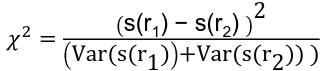
Direct Standardization Test-Based CI for sRR
Chi-square test for s(r1) = s(r2) is a variation on z test comparing two proportions:
Indirect Standardization
Used when rates in your population are not estimated well due to small sample sizes. We need :
- Crude rate in population/sample under study
- Strata distribution of popuation/sample under study
- Stratum-specific rates (and crude rates) for "standard" population
wi are the frequency from testing population and ri are rates from "standard" population.
- The stratum-specific rates in the study of interest are not reliable due to small sample size.
- Stratum-specific weights (wi) from population under study
- Strata distribution (ri) from "standard" population
- My weights, standard rates
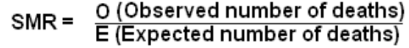
Results are often presented as a Standardized Mortality Ratio (SMR):
We can also calculate the standardized rate based on the standard population rate and teh target cohort-specific SMR:
s(r) = (Population Rate) x SMR
Indirect Standardization Test-Based CI for sRR
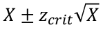
CI for an observed count using the Poisson model (SE = sqrt(mean)):
Standardized Estimators
All summary measures ignore non-uniformity and mask interaction, very similar to last chapter's tests for confounding with weights.
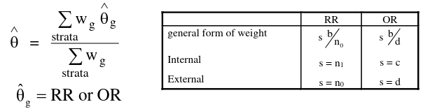
's' can also be weights (frequencies) derived from a standard population.
For RR:
- Internally Standardized
- s = n1 = exposed subjects sRR
- Externally Standardized
- s = n0 = unexposed subjects s'RR
For OR:
- Internally Standardized
- s = c = exposed non-cases sOR
- The interpretation of the OR would be something like: "If study participants who were not exposed to X have the same distribution of a confounding variable as those exposed to X who did not develop Y, then the increased odds of Y is OR for study participants exposed to X."
- s = c = exposed non-cases sOR
- Externally Standardized
- s = d = unexposed non-cases s'OR
- The interpretation of the OR would be something like: "If study participants have the same distribution of a confounding variable as those not exposed to X who developed Y, then the increased odds of Y is OR for study participants exposed to X."
Equivalent Estimators to the Standardized Risk Ratio:
- Directly standardized risk ratio with unexposed used as standard population
- Externally standardized RR
- SMR with unexposed as standard population
- Internally standardized RR
Test for Linear Trend in Odds Ratios
Test with several exposures, 2 * k tables (for association), or a series of 2 * 2 tables (for effect modification/interaction).
Note: Odds ratios are sensitive to non-linear transformations, but non-linear transformations can alter results.
Mantel Extension Chi-Square for 2 * k Tables
Let X = an ordinal score for exposure
H0: No linear (monotone) association between exposure and disease (proportion)
 with df = 1
And each stratum has variance:
Conclusion: We find a [de/in]creasing trend in incidence of [Outcome] with increasing levels of [independent] (p < .05), with ORs changing from OR_before to OR_after.
Test for Linear Trend in Odds Ratio for Several 2x2 Tables
The model we use is logarithmic: ln(OR) = b0 + b1X
We are testing H0: b0 = Odds Ratios for all tables OR All Odds Ratios are equal
Measure if there is an interaction present (ORs not all the same), or modelling interaction (ORs change systemically).
 with df = 1
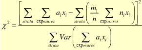
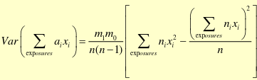
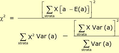
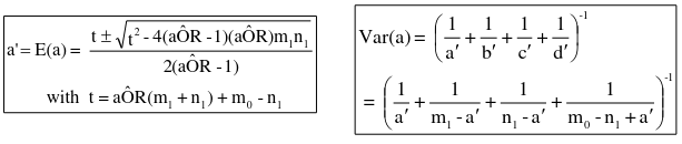
Where X is the score, and E(a) is the expected score under H0. E(a) and Var(a) can be computed as in the Test for homogeneity of Odds Ratios (Breslow-Day):
Matching
The aim of matching is remove confounding by matching subjects to be similar on a potential confounder. Doing so eliminates (or reduces) confounding, as well as reducing variability thereby increasing power.
Recall a paired t-test with two independent samples: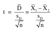
with n-1 degrees of freedom and standard error: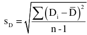
The test is inversely related to variance.
Types of Matching
- Matched Pairs (covered today)
- Categorical Matching (unmatched analysis, stratified or regression)
- Stratify cases, then find equal number of controls for each category (or equal multiple).
- Caliper Matching
- Only for continuous variables
- Similar to categorical but not the same
- Nearest Neighbor
- Select 'closest' control as match
- May have minimum match criteria
Matching in Follow-Up Study
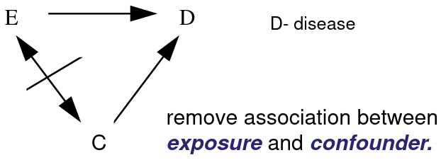
Remove Confounding (C) in the study sample between Exposed (E) and unexposed by matching on the potential confounders.
There are 4 possible combinations of outcomes in exposed and unexposed groups: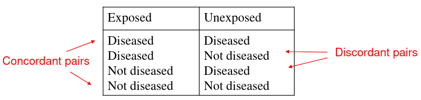
Corncordant pairs have the same outcome between pairs, and opposite in discordant pairs.
An example presentation for matching 2x2 tables: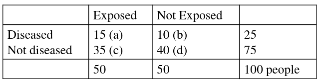
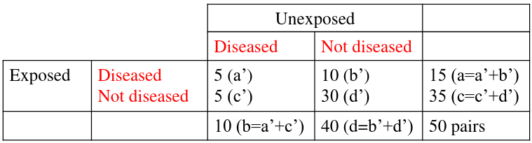
Notice the column and cell totals now equal the value of cells a,b,c,and d in the original table.
In the paired follow-up study table we would calculate the Relative Risk Ratio: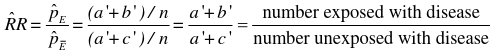
If we take the Risk Ratio of both the above tables, we find they are both the same (1.5).
Also, the confidence interval for RR in a follow up would be: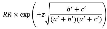
Matching in Case-Control Study
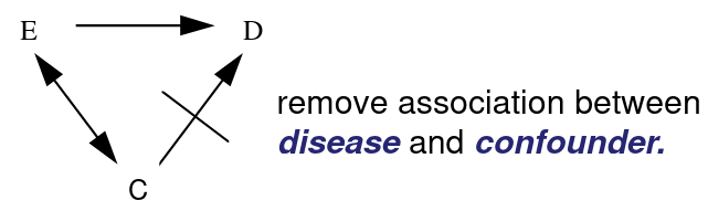
Remove Confounding (C) in the sample study between cases and controls by matching on potential confounders where for each case we select a control with the same values for the confounding variables.
For case control studies we set up our pairs differently:
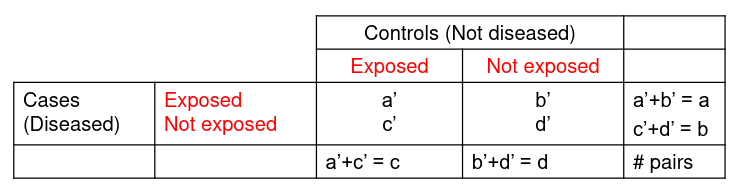
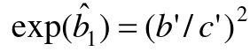
And this also result in a different estimate of Odds Ratio: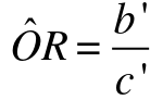
And likewise the confidence interval would be
OR x exp(+/- Z*sqrt(1/b' + 1/c')
ORs in Case-Control studies will not be the same if ignoring matching. This is unlike the situation for RR, where the point estimate is the same whether considering the matching or not.
The McNemar Test
The McNemar Test is a non-parametric test for paired nominal data. It is a chi-square distribution and can be used for retrospective case-control or follow-up studies. It assumes:
- The two groups are mutually exclusive
- A random sample
H0: The proportion of some disease is the same in participants with exposure and those without exposure (RR=1)
Ha: The proportion of some disease is not the same in participants with exposure and those without exposure (RR != 1)
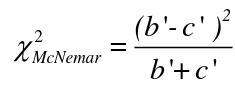 with df = 1
Matched Analyses and Mantel-Haenszel
Mantel-Haenszel methods applied to strata established by matched sets are equivalent to the conventional matched methods. Works for Cohort (Follow-Up) and case-control studies. When the matched pair is a stratum, we carry out the MH method on each pair.
So from the example above, if we calculated 50 strata for 50 matched pairs, we would end up with 50 tables:
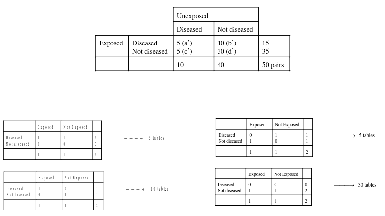
And then we apply the mRR and MH to each of the 50 strata to obtain the McNemar result.
Testing Interaction
It is possible to test interaction between a matching variable and exposure (whether a matching variable modified the effect of E on D).
We obtain an OR for each subgroup of the interaction variable and conduct a formal test to see whether the two ORs are equal.
R-1 Matching
Match one index to R referent subjects. We create a strata for every matched set. A stratum includes a matched set of R + 1 subjects.
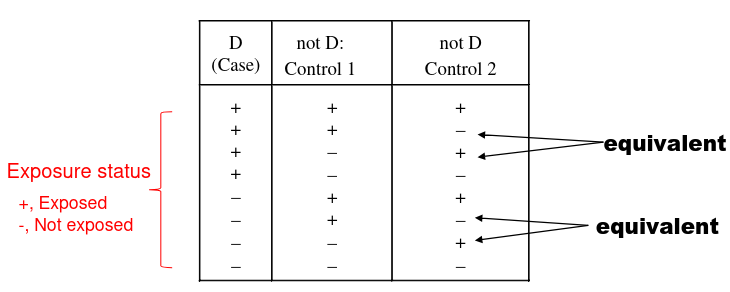
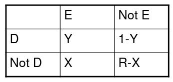
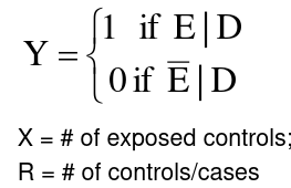
In a case control study:
- Index = case
- Referent = control
- Stratum:

- Exposure status:

- We can then use the following formulas for estimate of OR and chi-squared:

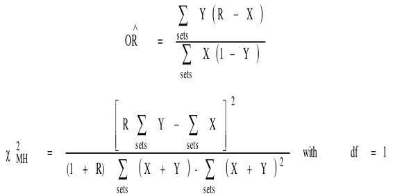
McNemar's test cannot be used in R-1 matching.
When to Match?
- How hard is it to obtain subjects?
- How hard is it to match?
- How much does matching buy?
- How influential are the confounders? How stronly correlated are the matched pairs?
- Is variation within the pairs small relative to variation between pairs?
- What do we gain?
- Eliminate/reduce confounding
- Reduce variability and increase power
Issues with Matching
- Matched studies use restriction sampling
- The exposed and the cases will not typically represent the general population
- Ex. a case-control study of smoking and lung cancer
- The cases will on average be more male and older than the general population and also may not reflect racial distribution
- We may not be able to generalize results
Code
### Matched pairs can be analyzed using the Mantel-Haenszel method.
### Each matched pair is treated as a separate stratum
mantelhaen.test(pairs$exposed, pairs$diseased, pairs$match, correct=FALSE)

# table of pairs:
table(exposed.d , unexposed.d)

### Analyze data with mcnemar.test()
mcnemar.test(table(exposed.d , unexposed.d), correct=FALSE)
mcnemar.test(table(exposed.d , unexposed.d))

### Matched sets can be analyzed using the Mantel-Haenszel method.
### Each matched set is treated as a separate stratum
mantelhaen.test(Rto1$smoke, Rto1$casecon, Rto1$casenum, correct=FALSE)
mantelhaen.test(Rto1$smoke, Rto1$casecon, Rto1$casenum)
Logistic Regression
Stratified analysis can be used to adjust for confounding, but the results can be difficult to adjust multiple confounders. If we have too many strata, we could end up with very small tables or 0 counts for some cells. We can instead use Logistic Regression when the following situation exists:
- The design is cross-sectional, case-control, cohort, or clinical trial
- The outcome (D) is dichotomous
- Any type of exposure (continuous, categorical or ordinal)
- Confounders/covariates can be continuous, categorical or ordinal
Goals of Logistic Regression
- Association: Between an outcome and a set of independent variables
- Prediction: What do we expect the probability of outcome to be given the set of independent variables?
- Exploratory: What variables are associated with outcome?
- Adjustment for Confounding: Focus on a particular relationship; the other variables in the model are there for adjustment
Properties of Exponential and Logarithmic Functions
- y = exp(x) -> log(y) = x
- exp(x)*exp(z) = exp(x + z)
- exp(x)/exp(z) = exp(x - z)
- log(a*b) = log(a) * log(b)
- log(a/b) = log(a) - log(b)
Logistic Regression Model
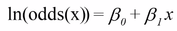
We assume a linear relationship between the predictor variable(s) and the Log-odds of an event that Y = 1:
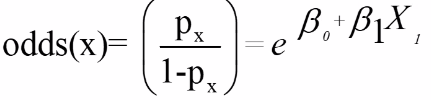
Thus, for risk p (if the design is appropriate):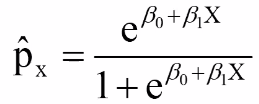
The predicted value of p is always between 0 and 1 and has a S-shaped curve.
Properties of Logistic Model with 1 Predictor: Case-Control Study
The log odds should be a straight line as given by: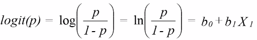
So if we have a X variable that is either 1 or 0 then the model would be:
logit(p | x = 0) = b0 or log(p | x = 1) = b0 + b1*1
With E being exposure and bar(E) being non-exposure, we can define the odds ratio as: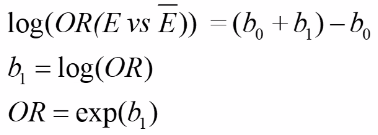
This represents the odds or log odds of developing disease with a dependent variable with one predictor in a case-control study.
In general: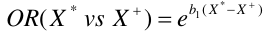
We can calculate confidence intervals for b: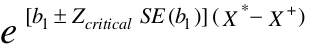
This will also hold true for more than one covariate in the model. But this is not true for the RR.
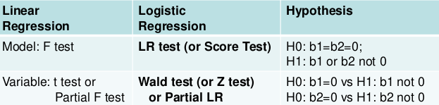
Testing the Model
Two levels of testing:
- Test of the model
- Test of specific variables in the model
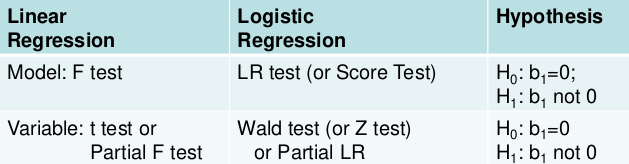
Likelihood Ratio Test
We can use the Maximum Likelihood test to estimate coefficients. Improvements in the likelihood by using the model with covariate instead of just the intercept. We use the Likelihood Ratio (LR) test when we do not know the distribution of LR.
H0: Model is x;
Ha: Model is x + all parameters
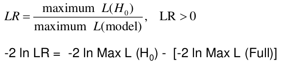
-2 ln(LR) has a chi-squared distribution with df = difference in number of parameters in the null and full models, assuming a large sample.
The LR, Wald, and Score test all measure the same hypothesis. For large sample sizes, they should all be equivalent. For small sample sizes LR is preferred.
LR test: 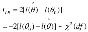
Score test: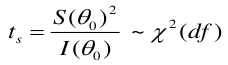
Wald test: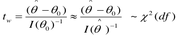
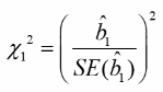
Multiple Covariates
As in multiple linear regression, the objective is to study the association by adjusting for confounding.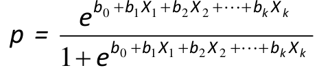
The joint effects of two independent variables is the multiplication of their individual effects (odds is the numerator from above).
We should remove missing values before analysis or apply other methods to consider missing data.
Partial Likelihood Ratio Test (PLRT) of a Specific Variable
PLRT is used to test the significance of a group of variables.
- Run model with all variables
- Run model with all except variable of interest
- Compare the model chi-square statistic or likelihoods, provided the sample sizes are the same
PLRT is almost equivalent to the Wald test. Often we use multiple dummy variables to code for a continuous covariate by putting the domain into "bins".
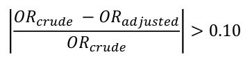
Confounding
Our measure of association for confounding: ORCrude / ORAdjusted
If the ratio is > 1.1 we conclude the factor confounds the association between X and Y.
In logistic regression the 10% rule of thumb should not be applied to beta.
R Code
#### This chunk of code
* reads data,
* extract records with complete data
* selects records for *FEMALES* and those with *CHD=0 OR CHD>4*
```{r }

framdat2 <- read.table("framdat2.txt",header=T, na.strings=c("."))
names(framdat2)

work.data <- na.omit(framdat2[,-c(3,4)]) ## drop DTH and CAU columns and remove rows with missing data
work.data <- subset(work.data, (work.data$SEX == 2) & (work.data$CHD==0 | work.data$CHD > 4))
work.data$chd_sw = work.data$CHD >= 4  ## 1 is event, 0 is no event
```

#### CRUDE ANALYSIS
We fit the model with only GLI, using the glm() function. "family=binomial" indicates that this is a logistic regression model.
```{r}

mod.crude <- glm(chd_sw ~ GLI, family=binomial, data=work.data)
summary(mod.crude)

```

##### Output for ORs, and Wald tests using the *aod* package
```{r }
confint.default(mod.crude)
exp(cbind(OR = coef(mod.crude), confint.default(mod.crude)))
library(aod) # inlcudes function wald.test()
wald.test(b = coef(mod.crude), Sigma = vcov(mod.crude), Terms = 2)
```

#### ADJUSTED ANALYSIS
model with only confounder
```{r }
mod.age <- glm(chd_sw ~ AGE, family=binomial, data=work.data)
summary(mod.age)
```

#### model fit and summary of parameter estimates - adjusted model
```{r }
mod.age.adjusted <- glm(chd_sw ~ GLI + AGE, family=binomial, data=work.data)
summary(mod.age.adjusted)
summary(mod.age.adjusted)$coefficients
```

##### to produce the LRT, use the anova function
```{r }
anova(mod.age, mod.age.adjusted)
```

##### estimate of adjusted OR and confidence intervals
```{r }
# regression coefficients
confint.default(mod.age.adjusted)

print( "Adjusted OR and 95% CI")
exp(cbind(OR = coef(mod.age.adjusted), confint.default(mod.age.adjusted)))
wald.test(b = coef(mod.age.adjusted), Sigma = vcov(mod.age.adjusted), Terms = 2)
```

##### Question: is there confounding?
```{r }
exp(coef(mod.crude)["GLI"])/exp(coef(mod.age.adjusted)["GLI"])
```

#### Interpretation of fitted values
```{r }
log.odds.CHD <- log(mod.age.adjusted$fitted.values/(1-mod.age.adjusted$fitted.values))
plot(work.data$AGE,log.odds.CHD,xlab="Age", ylab="log-odds-CHD")
points(work.data$AGE[work.data$GLI==1],log.odds.CHD[work.data$GLI==1],col=2)

odds.CHD <- mod.age.adjusted$fitted.values/(1-mod.age.adjusted$fitted.values)
plot(work.data$AGE,odds.CHD,xlab="Age", ylab="odds-CHD")
points(work.data$AGE[work.data$GLI==1],odds.CHD[work.data$GLI==1],col=2)

```

####  model with multiple confounders -- model fit and summary of parameter estimates
```{r }
mod.adjusted <- glm(chd_sw ~ GLI + AGE + CSM + FVC + MRW + SPF, family=binomial, data=work.data)
summary(mod.adjusted)
exp(cbind(OR = coef(mod.adjusted), confint.default(mod.adjusted)))
wald.test(b = coef(mod.adjusted), Sigma = vcov(mod.adjusted), Terms = 3)
```

##### fit model with only confounders
```{r }
mod.confounders <- glm(chd_sw ~ AGE + CSM + FVC + MRW + SPF, family=binomial, data=work.data)
summary(mod.confounders)
anova(mod.confounders,mod.adjusted)
```
Logistic Regression in Matched Studies
In case-control studies matching cases and controls on a potential confounder improves the efficiency of a study and removes/reduces bias.
Logistic regression controlling for a stratification variable allows us to examine multiple risk factors and control for confounders that where not matched, which is advantageous over the Mantel-Haenszel for stratified analysis.
Conditional Logistic Regression
Treats the strata effect as 'nuisance parameters'; controls for the strata but does not estimate effects. Uses 'conditional likelihood' to fit the model. Estimates effects of other parameters within strata by pooling across strata.
We can analyze the data in two ways: Matched pairs or as matched sets. Where matched pairs are always cases matched with 1 control, in matched sets the case can be matched with up to four controls. Matching conditionally on pairs in called conditional analysis.
Unconditional Model (Wrong Way)
Consider a logistic function with many strata:
These stratum effects are nuisance parameters which contribute to the baseline risk in each stratum: b0 + bi
The MLE maximizes this function: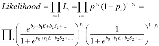
It can be shown the the odds ratio based on the MLE of b1.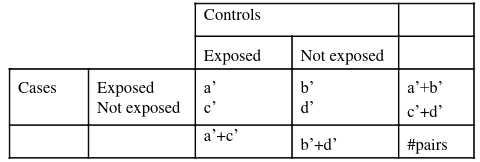
So running the above without matching gives use the wrong results. Thus, this analysis is NOT APPROPRIATE with matched pair data. We never use unconditional logistic regression for matched pairs or sets.
Correct Approach
Uses conditional likelihood approach to focus only on parameters of interest. Nuisance parameters are "conditioned" out of the analysis; no nuisance parameters in the likelihood.
Only informative strata contribute to the likelihood: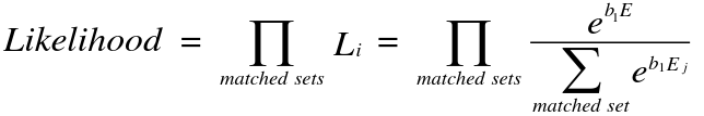
Maximum Likelihood Estimation uses likelihood on matched sets instead of individuals. We adjust for variables not matched within the matched set, or variables that cannot be practically adjusted for in regression.
Matching introduces some dependencies between subjects that cannot be ignored across strata.
Also note the Breslow-Day test has no meaning in matched sets analysis.
R Code
library(survival)

### Create variables
match <- c()
for(i in 1:63){ match <- c(match, rep(i,2))}
disease <- rep( c(1,0), 63)                          ## each pair has exposed/unexposed
exposed <- c(rep(c(1,1), 27),                        ## 27 pairs (D, E), (not D, E)
                        rep(c(1,0),                  ## 29 pairs (D, E), (not D, not E)
                        rep(c(0,1), 3),              ## 3 pairs (D, not E), (not D, E)
                        rep(c(0,0), 4))              ## 4 pairs (D, not E), (not D, not E)


### Unconditional Model - INCORRECT
mod <- glm(disease ~ exposed + factor(match), family = binomial)
summary(mod)

### Conditional Logistic Regression - CORRECT
mod <- clogit(disease ~ exposed + strata(match))
summary(mod)


### Estrodat data
## Read the data ##
estrodat <- read.csv("estrodat.csv", header=T, na.strings=".")
estrodat2 <- subset(estrodat, is.na(age)==F & is.na(gall)==F & is.na(hyper)==F
                    & is.na(obesity)==F)
m.uni <- clogit(case ~ estro + strata(match), data = estrodat2)
summary(m.uni)

m.multi <- clogit(case ~ estro + age + gall + hyper + obesity + strata(match), data = estrodat2)
summary(m.multi)

### Uninformative sets
uninform.index <- c()
for (i in 1:length(unique(estrodat2$match))) {
  if (length(unique(estrodat2$case[ which(estrodat2$match==i)])) < 2) {
    uninform.index <- c(uninform.index, i)
  }
}
estrodat2[ which(estrodat2$match %in% uninform.index),]

estrodat3 <- estrodat2[ -which(estrodat2$match %in% uninform.index),]
### Crude Analysis
m.uni2 <- clogit(case ~ estro + strata(match), data = estrodat3)
summary(m.uni2)

m.multi2 <- clogit(case ~ estro + age + gall + hyper + obesity + strata(match),
data = estrodat3)
summary(m.multi2)
Survival Analysis I
Survival analysis is a measure of time until an event occurs. It doesn't only measure death as an outcome, and can adjust for covariates just as a logistic regression. But while a logistic regression only requires knowledge of whether an outcome occurred, survival analysis requires knowledge of the time until the outcome occurred.
This is usually used in a longitudinal cohort study; not common in case control studies as there is no accurate time information.
Survival Data
Survival data contains: entry time, whether the person had the event (dichotomous), and the time between when the person had the event or was last known to be event-free; as well as any other covariates (race, gender, age, etc).
Even those who drop out of the study before the outcome occurs can provide information to the study. They are assumed to have the same likelihood of death as subjects with similar characteristics who survived at least the same amount of time.
Censoring
Censoring is removing a subject before we can measure the outcome.
Type I Censoring: Observations censored after some fixed length of follow-up.
Type II Censoring: Observations censored after a fixed percentage of subjects have the event of interest.
Random Censoring: Observations censored for reasons outside the control of investigators (e.g. drop-outs).
Informative Censoring: People censored that would have had different outcomes as people who remained in the analysis for the same amount of time.
Non-informative Censoring: People censored who would have had similar risk for the outcome as people who remained in the analysis for the same amount of time. Basic survival analysis assumes that censoring is non-informative.
Right-Censored: Lower limit on the time to an event for censored subjects (more common)
Left-Censored: An upper limit on time to event (less common, also called interval-censored with both upper and lower limits)
Survival Analysis vs. Alternatives
Linear Regression
If we have a continuous dependent variable, there are several issues with using a linear regression with time to event or censoring as outcome:
- Censored observations can't be incorporated
- Distribution of survival time is usually highly skewed since some people nearly always survive a long time
- Disease status can't be handled
Logistic Regression
Neither time to event nor censoring are relevant in a logistic regression; the time between exposure and outcome is very short, and people cannot "drop out" of the study since they are recruited after the outcome is known.
Survival Function
Measures: Let T = survival time to event
Survival probability: S(t) = Pr (T > t) = Pr(the probability that an event has NOT occurred until time 't')
- S(t=0) = 1 (all survive at the start)
- S(t=inf) = 0 (non-one survives at infinity time)
- 0 <= S(t) <= 1
- S(t) is non-increasing function S(t1) >= S(t2) for t1 <= t2
Failure Function
T = survival time to event
Failure probability - the probability that event occurred by time 't'
F(t) = Pr(T <= t)
Relationship between survival function and failure function S(t) = 1 - F(t)
Hazard Rate
Instantaneous failure rate
$$ h(t) = \lim_{\Delta t \to 0 } {{Pr(t < T \le t + \Delta t | T > t)} \over {\delta t}} $$
$$ H(t) = \int h(t)*d(t) $$
Relationship between hazard and survival functions:
$$ h(t) = {f(t)} \over {S(t)} $$
f(t) = density of time to event
Cumulative hazard = H(t) = -ln(S(t))
Kaplan-Meier Curves
Kaplan-Meier curves (AKA Product-Limit Estimate) is a non-parametric approach. No assumptions on shape of the underlying distribution for survival time.
Example with censoring: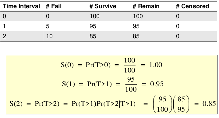
Example with censoring: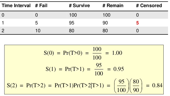
Summary Measures
- Median survival - smallest survival time for which S(t) < .5
- Sometimes this cannot be estimated
- Mean survival
- Often biased
- Hazard Ratio - cannot be estimated from the KM curve and it depends on the proportional hazards assumption
Log-Rank Test
A non-parametric crude comparison among several groups. Test whether two survival curves are statistically different by comparing observed events with expected events under the null hypothesis of no difference. Can be thought of as a time-stratified C.M.H. test.
H0: There is no difference between the populations in the probability of an event at any point in time
At the jth failure time: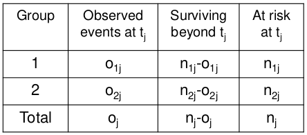
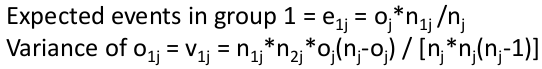
Where o = observed and e = expected
Total observed events in group 1: O1 = Sum of o1j for all j
Total expected events in group 1: E1 = Sum of e1j for all j
Variance of O1 = sum of v1j for all j
Log Rank Statistic: (O1 - E1)2 / V ~ X2 (1 df)
Proportional Hazards
An assumption of the Log-Rank test is "proportional hazards", that the hazard functions in different groups are proportional.
The survival distributions crossing is an indication of the non-proportional hazards.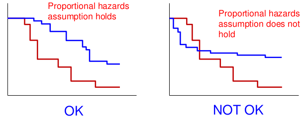
In the next chapter we will learn a formal test for proportional hazards
Regression Models for Survival Analysis
Kaplan-Meier estimator allows for crude comparison, but it does not provide an effect estimate nor does it allow adjustment for covariates.
We model the hazard as a function of the exposure and quantify the relative hazard. The hazard ratio is the effect estimate, and it allows adjustment for covariates.
T = time to event
Survival Distribution: S(t) = Pr(T > t) = Pr(Subject survives at least to time t)
Hazard function: Instantaneous failure rate, event rate over a small interval of time. Not a probability, can be greater than 1.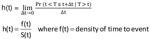
Proportional Hazards Models
The exponential model describes the hazard function as:
= basline hazard * effect of covariates
baseline hazard is a constant (it does not change with time)
R Code
### KM Curves and Log-Rank Test
fit.2 <- survfit(Surv(chdtime, chd_sw) ~ GLI, data=framdat3)
summary(fit.2)

# Kaplan-Meier Plot
plot(fit.2, mark.time=T, mark=c(1,2), col=c(1,2), lwd=2, ylim=c(0,1),
             xlab="Time (years)", ylab="Disease free survival", cex.axis=1.5, cex.lab=1.5)
legend(x=1, y=0.40, legend=c("No GLI","GLI"),
             col=c(1,2), lwd=2, cex=1.2)

# Log-Rank Test
survdiff(Surv(chdtime, chd_sw) ~ GLI, data=framdat3)

### A fancier survival plot using the **survminer** package
#### Reference https://rpkgs.datanovia.com/survminer/index.html
library(survminer)
ggsurvplot(
  fit.2,
  data = framdat3,
  xlab="Time (years)",
  size = 1,                 # change line size
  palette =
    c("#FF3333","#0066CC"),       # custom color palettes
  conf.int = TRUE,          # Add confidence interval
  pval = TRUE,              # Add p-value
  risk.table = TRUE,        # Add risk table
  risk.table.col = "strata",# Risk table color by groups
  legend.labs =
    c("GLI=0", "GLI=1"),    # Change legend labels
  risk.table.height = 0.3,  # Useful to change when you have multiple groups
  ggtheme = theme_bw()      # Change ggplot2 theme
)
Survival Analysis II
In survival data the dependent variable is always survival time (or time until an event with the potential to censor observations). The independent variable can be any type; Continuous, ordinal or categorical. We assume the observations are independently and randomly drawn from the population.
Kaplan-Meier estimator allows crude comparison between two groups, but it does not provide an effect estimate or allow adjustment for covariates.
Cox Proportional Hazards Model
In 1972 Sir David Cox introduced a survival model in which the hazard function changes with time only through the baseline function.
We can model the hazard as a function of the exposure and quantify the relative hazard, which allows for adjustment of covariates. This is the instantaneous failure rate, or the event rate over a small interval or time. The hazard ratio does not depend on time. The hazard baseline function is modeled as: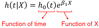
A hazard ratio at time t for a change in X: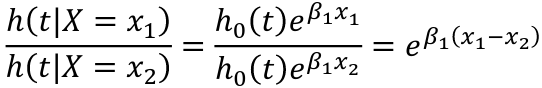
The baseline hazard function, h0(t) when X=0, is treated as a nuisance function and is left unspecified (non-parametric part of the model). The covariates affect the hazard function multiplicatively through the function exp(Beta*X) (the parametric part of the model).

The model is therefore called a semi-parametric model. It is suitable when we are more interested in the parameter estimates (effects of covariates) than the shape of the hazard. Fit by maximizing the partial likelihood.
X = 0![]()
X = 1![]()
Hazard ratio X=1 vs X=0![]()
![]()
CI is similar to logistic regression, we only model the hazard rather than the odds. Situations in which you might expect the logistic and PH regression results to differ:
- Common event (cumulative risk for the event is not small)
- Differential loss to follow-up (loss differs by exposure)
- Exposures change over follow-up
Tied Event Times
- Breslow's Method
- An approximation to the exact adjustment
- Default option in SAS
- Efron's method
- A different approximation to the exact adjustment
- A better approximation than Breslow's method
- Default in R / SAS: "ties=efron" in PROC PHREG
- Kalbfleisch and Prentice's "exact" method
- Assumes ties are due to imprecise measurement of time
- Most computationally-intensive method (all possible ordering of tied data is considered)
- Not available in R / SAS: "ties=exact" in PROC PHREG
All will give the identical estimates if there are no ties.
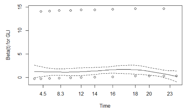
Proportional Hazards Assumption
Beta should not change with time if the proportional hazards assumption holds.
H0: Proportional hazard is satisfied
Conclusion: We fail to reject the null hypothesis, so no evidence of departure from the PH assumption
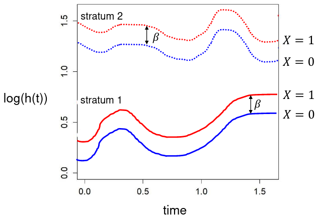
- Graphical Method: log(-log(S(t))) plot
- The natural logs of h(t | X) plotted against time are parallel for varying values of X, separated by Beta
- Likewise, the log of the negative log of S(t | X) plotted against time (or log(time)) are parallel for varying values of X, separated by Beta

- Schoenfeld Residuals
- Suppose subject i has an event at time tt
- The Schoenfeld residual for subject i and covariate X is:
- xi - x_bar(ti), where x_bar(ti) is the estimated mean of X based on the subjects at risk at time ti (similar to observed - expected)
- A test of the PH assumption is based on a test of the correlation between sccaled Schoenfeld residuals and a function of time
- If the PH assumption is satisifed the Schoenfeld residuals should be uncorrelated with time
- A significant test (small p-value) suggests that the PH assumption fails
- If the proportional hazards assumption is satisfied the plot should look like a horizontal line
- In R: 'cox.zph(linreg)'

- Time-varying Effects
- SAS and R have internal algorithms to build the "time-varying covariates", this is NOT the same as including a time covariate interaction in the model.
- In this method we think of Beta as a function of time:
Beta = a + bt

- Martingale Residuals (SAS Only)
- Using ASSESS statement in SAS
- Assess both functional form and proportional hazards assumption for each covariate using simulation
- A set value needs to be set to reproduce results
- The observed path (solid line) should not be extreme compared to the simulated paths (dashed lines)


Which Test to Use?
A method should be choosen ahead of time. Tests based on Schoenfeld residuals and time-varying effects are the most commonly reported.
Non-Proportional Hazards
If the variables failing PH assumption are not of interest we can use a stratified PH model in which a different baseline hazard is fitted per stratum.
If the variables failing PH assumption are of interest include the time-dependent variable and deal with complicated conclusion of HR varying over time. This can be hard to interpret.
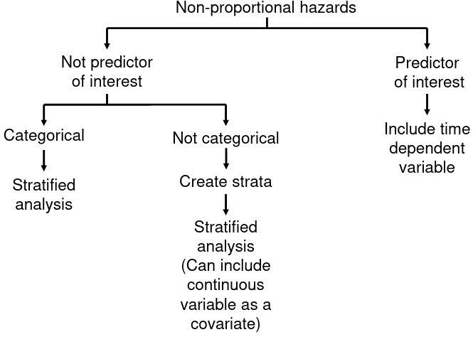
Defining Strata
Each stratum use a separate baseline hazard: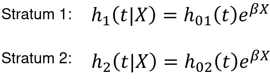
The Beta is the same for each stratum and the effect of the variable is now part of the baseline hazard.
For example, if we create stratum based on sex, we can no longer use the model to compare hazards across sex, as the effect of sex is now part of the baseline hazard, which we do not estimate.
We compare the exposed subjects to unexposed subjects within the same stratum. We cannot compare exposed subjects to unexposed subjects across different strata.
Stratifying Continuous Variables
- Create a categorical variable defining strata based on the continuous variable
- Use this categorical variable to stratify the analysis
- Include the continuous variable as a covariate in the model to account for residual association within the strata. Results are difficult to interpret
You can keep an interaction between X and time in your model if it failed the PH assumption, but you cannot interpret the parameter estimate since it is a function of time.
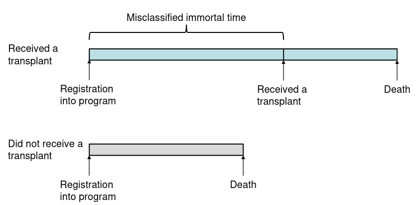
Time-Dependent Exposures
Some exposures vary over time, and this varying exposure is important to assess. The Cox model can be extended to accommodate this. For example, someone who has been smoking since they were young has different survival rate compared to someone who just started smoking.
Immortal Time Bias - Effect of an exposure can be biased toward survival if there is a delay between entry into study and exposure.
R Code
library(survival)
framdat4 <- read.csv("framdat4.csv", header=T, na.strings=c("."))

## Cox Proportional Hazards regression
### Crude Model

# Fit the model: coxph()
fit.1 <- coxph(Surv(chdtime, chd_sw) ~ GLI, data=framdat4)
summary(fit.1)


### Adjusted Model
fit.2 <- coxph(Surv(chdtime, chd_sw) ~ GLI+AGE+SPF+CSM+FVC+MRW, data=framdat4)
summary(fit.2)

## Assess the PH assumption
### Log(-Log(Survival)) Plot
fit.km <- survfit(Surv(chdtime, chd_sw) ~ GLI, data=framdat4)

# Method 1: use the fun="cloglog" option
plot(fit.km, col=c("black", "red"), fun="cloglog",  main="Log of Negative Log of Estimated Survival",
     xlab="time", ylab="log(-log(survival))", cex.main=1.5, cex.axis=1.5, cex.lab=1.5)
legend(x=12, y=-3.5, legend=c("No GLI","GLI"), col=c(1,2), lwd=1, cex=1.2)

# Method 2: calculate the logs manually
plot(log(fit.km$time),log(-log(fit.km$surv)), main="Log of Negative Log of Estimated Survival",
     xlab="log(time)", ylab="log(-log(survival))", cex.main=1.5, cex.axis=1.5, cex.lab=1.5)
lines(log(fit.km$time[1:12]), log(-log(fit.km$surv[1:12])), lwd=2)
lines(log(fit.km$time[13:24]), log(-log(fit.km$surv[13:24])), lwd=2, col=2)
legend(x=2.5, y=-3.5, legend=c("No GLI","GLI"), col=c(1,2), lwd=2, cex=1.2)

### Schoenfeld residuals
# Assess the PH assumption: cox.zph()
test.1 <- cox.zph(fit.1)
print(test.1)
plot(test.1)

test.2 <- cox.zph(fit.2)
print(test.2)
plot(test.2)

### Time-Varying Covariates to assess PH assumption
# Use the 'tt' option
# (1) Interaction with time
fit.a <- coxph(Surv(chdtime, chd_sw) ~ GLI+tt(GLI), data=framdat4,
                   tt=function(x,t,...)x*t)
summary(fit.a)
# plot HR
plot(c(0:25), exp(1.46-0.024*c(0:25)), type="l", xlab="Time (years)", ylab="HR", col="blue", lwd=2)

# (2) Interaction with log(time)
fit.b <- coxph(Surv(chdtime, chd_sw) ~ GLI+tt(GLI), data=framdat4,
                   tt=function(x,t,...)x*log(t))

summary(fit.b)
# plot HR
plot(c(0:25), exp(1.28-0.05*log(c(0:25))), type="l", xlab="Time (years)", ylab="HR", col="blue", lwd=2)

### Stratified analysis
# Create age strata
age.group <- rep(1, nrow(framdat4))
age.group[ which(framdat4$AGE >44 & framdat4$AGE <55)] <-2
age.group[ which(framdat4$AGE >54 & framdat4$AGE <65)] <-3
age.group[ which(framdat4$AGE >64 & framdat4$AGE <75)] <-4

# Fit stratified model using strata() option
fit.s <- coxph(Surv(chdtime, chd_sw) ~ GLI+SPF+CSM+FVC+MRW+AGE+strata(age.group),
               data=framdat4)
summary(fit.s)

cox.zph(fit.s)
Model Fit & Concepts of Interaction
Review: Logistic and Proportional Hazards Regression Model Selection
You can look at changes in the deviance (-2 log likelihood change)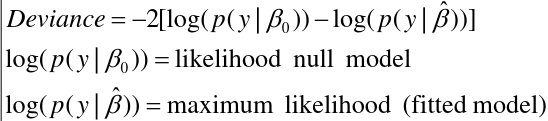
- Deviance - Residual sum of squares with normal data
- Problem: Deviances alone do not penalize "model complexity" (hence need LRT - but only applies to nested models)
- AIC, BIC - More commonly used
- Larger BIC and AIC -> worse model
- BIC is more conservative
- Both based on likelihood
- An advantage is that you do not need hierarchical models to compare the AIC or BIC between models
- A disadvantage is there is no test nor p-value that goes with comparison of models
- A model with smaller values of AIC or BIC provides a better fit
- Used to compare non-nested models
- A non-nested model refers to one that is not nested in another; The set of independent variables in one model is not a subset of the independent variables in the other models
- The data must be the same
Risk Prediction and Model Performance
How well does this model predict whether a person will have the outcome? Generally only for dichotomous outcomes, especially in genetics.
- Calibration - Quantifies how close predictions are to actual outcomes - goodness of fit
- Models for which expected and observed event rates in subgroups are similar are well-calibrated
- Discrimination - The ability of the model to distinguish correctly between the two classes of outcome
Logistic
- A model that assigns a probability of 1 to all events and 0 to non-events would have perfect calibration and discrimination
- A model that assigns a probability of .51 to all events and .49 to all non-events would have perfect discrimination and poor calibration
Hosmer-Lemshow Test
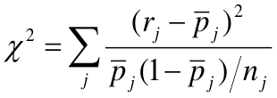
The Hosmer-Lemshow Test is a statistical goodness of fit test for logistic regression models. It is frequently used in risk prediction models. It assesses whether or not the observed event rates match expected event rates in subgroups of the model population of size n. Specifically, it identifies subgroups as the deciles of size nj based on fitted risk values.
H0: The observed and expected proportions are the same across all groups
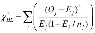
- Oj and Ej refer to the observed events and expected events respective in the jth group
- nj refers to the number of observations in the jth group
- Sensitive to small event probabilities in categories
- Sensitive to large sample sizes
- Problems: Results immensely depend on the number of groups and there is no theory to guide the choice of that number. It cannot be used to compare models.
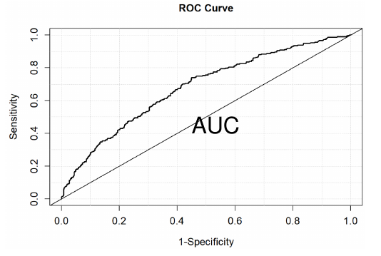
ROC: Receiver Operating Curve / C Statistic
Plots sensitivity (true positive) for different decisions and look for best trade off between sensitivity and specificity (true negative). The curve is generated using signal detection applications.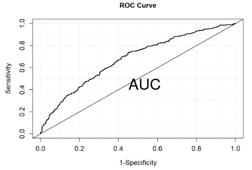
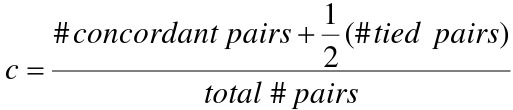
The area under the curve (AUC) is a summary measure called the c statistic, which is the probability that a randomly chosen subject with the event will have a higher predicted probability of the event than a randomly chosen subject without the event (a measure of discrimination).
- > .8 - very good
- > .75 - good
- > .7 - acceptable
- > .65 - weak
- > .6 - poor
- < .6 - useless
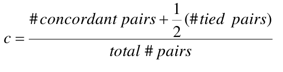
The c statistic groups all pairs of subjects with different outcomes and identifies pairs where the subject with the higher predicted value also has the higher outcome concordantly. Pairs where the subject with the higher predicted value has the lower outcome are discordant.
When we use the c-statistic in the data used to build the model it cannot be interpreted as the "true" predictive accuracy. It is simply a measure of goodness of fit.
Real predictive accuracy can be estimated when you have a new data set that is not used to generate the model. If that is not possible, inter-validation can be considered:
- Random split - Random splitting of the sample into training and validation many times (100+)
- Cross-validation - Dividing the sample into k sub-samples and train the model on k-1 samples then validate on the remaining sample and repeat many times
- Bootstrap - Resampling with replacement a new version of your sample, where each observation has the same probability of selection. The new sample is used for analysis many times
Survival Analysis
- Calibration at large - compares how close the mean of the model-based predicted probabilities at time t is to the Kaplan-Meier estimate at time t
- Calibration by decile - replace rates/proportions in deciles with their Kaplan-Meier equivalents; change degrees of freedom to 9
- c-statistic has several extensions to survival data, the most popular is Harrell's:
- Call any two subjects comparable if we can tell which one survived longer
- Call two subjects concordant if they are comparable and their predicted probabilities of survival agree with their observed survival times
- 'c' defined as the probability of concordance given comparability
Interaction Analysis
Interaction is when the effect of an exposure depends on the presence or absence of another exposure, or on the level of another exposure variable.
- If there is an interaction:
- We say there is an interaction between the two exposures
- We cannot provide a single summary measure
- A treatment may be beneficial to some subgroups but harmful to other subgroups
- Sometimes helps clarify the mechanisms for outcome
- When the interaction is model dependent:
- Evaluation of interaction depends upon the measures you are using to examine the association between exposure and disease
- Risk differences vs ratio measures lead to different concepts of interaction
Effect Modification
There is a difference between interaction and effect modification but I will not go into detail here.
One 'exposure' is a non-modifiable background variable such as a demographic variable (a 'moderator'). The moderator affects the size and/or direction of the association between a primary exposure and an outcome.
Ex. Sex may be a moderator of the association between hypertension and heart disease, as reflected by the difference in risk ratios between men and women.
Statistical vs. Biological Interaction
- Biological interaction, or mechanistic interaction, is when two exposures are part of the same causal mechanism
- Statistical interaction is interaction in a statistical model (the focus below)
- It is model and scale dependent: a model for risk differences may indicate an interaction while a model for risk ratios indicates no interaction, or vice versa
- The presence of a statistical interaction does not mean there is necessarily any mechanistic or biological interaction
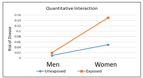
Quantitative Interaction
Quantitative interaction is when the direction of the effect of an exposure on an outcome is the same for different subgroups but the size of the effect differs.
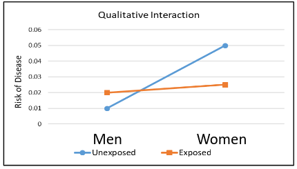
Qualitative Interaction
Qualitative interaction is when the direction of the effect of an exposure on an outcome changes for different subgroups.
Additive Interaction
Note: In the following sections we ignore sampling variability. We'll assume we have very, very large samples or an entire population.
Suppose we have two binary exposures A and B with risk: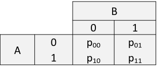
There is interaction on the additive scale if the effect of the two exposure together is not equal to the sum: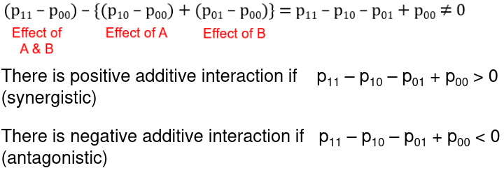
Example: Suppose we have two binary exposures A and B that have the following risk table: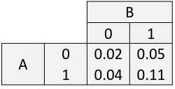
The risk difference compared to those with neither exposure: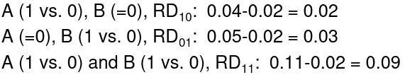
Note that RD11 > RD10 + RD01 (Synergistic)
Risk Ratio Difference
Recall that a risk ratio of 1 means no risk.
For risk ratios: There is an interaction on the additive scale if the effect of the two exposures together is not equal to the sum of their individual effects: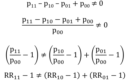
Thus, there is an interaction on the additive scale if the deviation from 1 (the null value) of the risk ratio for both exposures is not equal to the sum of deviations from 1 of the individual risk ratio for each exposure separately.
The important thing to remember here is the additive interaction can be assessed based on risk ratios without the having underlying risks.
Relative Excess Risk Due to Interaction
So there is not interaction on the additive scale if:
The quantity, R11 - R10 - RR01 + 1, is called the relative excess risk due to interaction or RERI:
There is interaction on the additive scale if the RERI != 0
> 0 means positive additive interaction
< 0 means negative additive interaction
Multiplicative Scale
Suppose we have a table of risks similar to the additive risk above.
There is an interactive on the multiplicative scale if the effect of the two exposures together is not equal to the product of their individual effects:![]()
It is possible to have both additive and multiplicative interaction, or a positive additive interaction and negative multiplicative interaction.
Case Control Studies
Additive Scale
If the outcome is rare, so that ORs estimate RRs, then we can say there is additive interaction if:![]()
We can define the relative excess risk due to interaction as:
There is interaction on the additive scale if RERI != 0
> 0 means positive additive interaction
< 0 means negative additive interaction
Multiplicative Scale
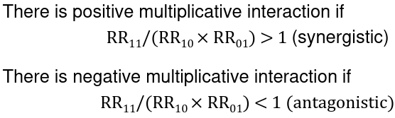
In this setting multiplicative interaction exists when:
OR_11 != OR1_10 * OR_01
OR_11 / OR1_10 * OR_01
> 1 means positive multiplicative interaction
< 1 means negative multiplicative interaction
Note this is only based on odds ratios, there is no multiplicative interaction between risk ratios, unless the outcome is rare and ORs approximate RRs.
Additive vs Multiplicative Interaction
- Direction of interaction may depend on the scale
- If both exposures affect the outcome then there is necessarily interaction on one of the scale
- There is no interaction on either scale then one of the exposures must have no effect on the outcome
- It is argued additive interaction is the more important public health measure
Modeling with Interaction
Hierarchical models always have the lower order terms before considering higher order terms
Ex. Hierarchical: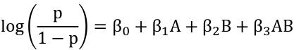
Ex. Non-Hierarchical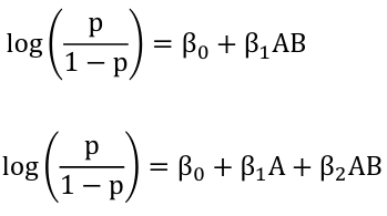
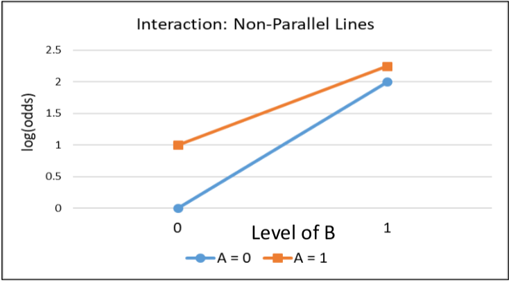
When there is no interaction term in a model the log(odds ratio) remains constant.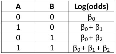
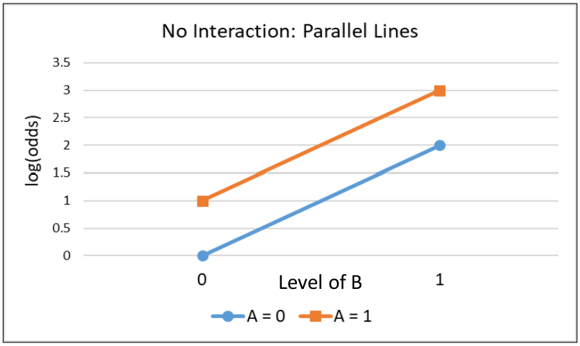
When there is an interaction term the log odds ratio is NOT constant. There is also interaction on the multiplicative scale.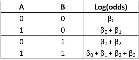
Synergy: If beta_3 > 0 the joint effect of A and B is greater than the product of the individual effects.
Antagonism: If beta_3 < 0 the joint effect of A and B is less than the product of the individual effects.
The odds ratios (the group with neither exposure as the reference):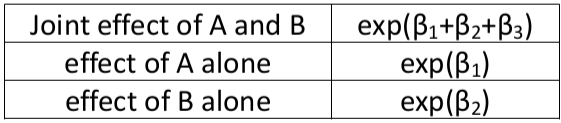
If there is an interaction term, the main effects cannot be interpreted alone, but are relative to the state of other variables.
R Code
library(effects) # To plot interactions
library(survival) # load survival package

# Hosmer-Lemshow Test
mod <- glm(y~x, family=binomial)
hl <- hoslem.test(mod$y, fitted(mod), g = 10)
Poisson Regression
We use the Poisson Regression to model a risk ratio when we are interested not in whether something occurs but how many times it occurs; Either repeated events or events in a population.Ex. number of hospitalizations, number of infections, etc.
This assumes independent events and equal risk over time (flat hazard)
Logistic regression produces odd ratios (which approximates risk ratio when outcome is rare), but only analyzes patients with at least 1 event and can be difficult to interpret when outcome is not rare. Survival analysis can be used to analyze the time to the first event.
Poisson Distribution
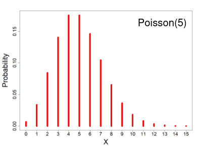
- X ~ Poisson(μ); μ > 0
- X = the number of occurrences of an event of interest, with parameter μ
- Probability mass function

- E(X) = μ
- V(X) = μ
The distribution depends of the expected number of events, since the mean = variance. As the number of expected number of events increases it the more closely the Poisson distribution approximates the normal distribution.
If X ~ Binomial(n, p) and n -> inf, p -> 0 such that np is constant; X ~ Poisson(np)
Distribution of the sum of independent Poisson random variables. If Xi ~ Poisson(μi) for i = 1 to m, and the Xi's are independent then: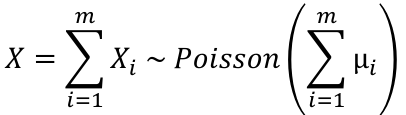
IR = (number of events)/(number of controls OR interventions)
Incident Rate Ratio = IR_intervention / IR_controls
CI for expected number of events (μ):
μL, μU = X +/- 1.96 * sqrt(X)
CI for Incidence Rate: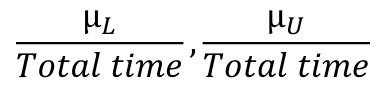
The event rate can also be written as:
λ = μ / N
Where μ is the expected number of events and N is the number of exposure units
We model the relationship on the log scale: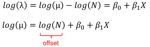
So to use the Poisson model we need 3 things:
- Predictor variables and covariates X1, X2, X3...
- The number of events for each "subject", defined as the group to which the event count belongs
- The denominator that the events are drawn from Ni
For specific values of X, X*, X+:![]()
For a CI for IRR(X* vs X+):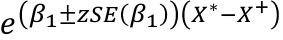
Overdispersion
Overidispersion is when the variance is greater than the mean, and is a significant problem for Poisson regression. Outliers can lead to large variances, and unmeasured effect modifications and confounders. Uncontrolled overdispersion results in model where the p-values are too small.
The solution is scaling the data to fix the standard error, the estimate is unchanged but the p-value is fixed.
Alternatives
Negative Binomial Regression
Evidence of under-dispersion (small deviance) or overdispersion (large deviance) indicates inadequate fit of the Poisson model or improper variance specification. Mean = variance requires a homogenous population, having a heterogenous population will introduce additional variance.
NBR is used in cases where there is overdispersion in a Poisson regression:
Variance = mean + k*mean^2 (k>=0)
The negative binomial distribution reduces to Poisson when k = 0; Where k is the number of variables.
We can test if the NBR fits the data better than the Poisson regression. One such way is a likelihood ratio test (LRT):
- Run the first model with K variables, and record the -2Log Likelihood
- Run the second model with K+P variables and record the -2Log Likelihood
- Calculate the difference in the -2Log Likelihood
- The difference is the chi-sqaure distributed with P degrees of freedom
H0: k = 0; Ha: k>0
Zero-Inflated Poisson Models
In cases where the number of subjects with no events exceeds the expected we can consider a model where we split analysis into 2 parts:
- Look at the probability of events vs none using logistic regression
- Given at least one event, model the number of events using Poisson regression model
- The logistic and Poisson model parts are estimated at the same time
- The risk factors for having any events don't have to be the same risk factors that predict how many events happen
This will not be covered in detail here.
Risk Ratio Regression
Epidemiologists prefer risk ratios over odds ratios, as they are more intuitive. It is argued since the odds ratio estimates the risk ratio when the outcome is rare there is no good justification for fitting logistic regression models to estimate odds ratios, log binomial or Poisson are greatly preferred.
Logistic regression models the odds: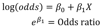
Log-binomial can be used to model the risk: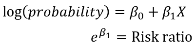
Note that the log of a probability is always negative.
- Generally log-binomial and Poisson regression models appear to have difficulties when prevalence is high (when odds ratios and risk ratios are most different).
- Poisson regression models are somewhat sensitive to outliers
- Log binomial models are very sensitive to outliers
R Code
library(epitools)
library(aod) # For Wald tests
library(MASS) # for glm.nb()
library(lmtest) # for lrtest()
library(gee) # for gee()
library(geepack) # for geeglm()

## Poisson regression
### Import data
patients <- read.csv("patients.csv", header=T)


### Poisson regression: crude model
mod.p <- glm(NumEvents ~ Intervention, family = poisson(link="log"), offset = log(fuptime), data=patients)
summary(mod.p)
confint.default(mod.p)
exp(cbind(IRR = coef(mod.p), confint.default(mod.p)))

### Poisson regression: adjusted model
mod.p2 <- glm(NumEvents ~ Intervention + Severity, family = poisson(link="log"), offset = log(fuptime), data=patients)
summary(mod.p2)
exp(cbind(IRR = coef(mod.p2), confint.default(mod.p2)))

### Poisson regression with summary data
Intervention <- c(0,1)
NumEvents <- c(481,463)
fuptime <- c(876,1008)

mod.s <- glm(NumEvents ~ Intervention, family = poisson(link="log"), offset = log(fuptime))
summary(mod.s)
exp(cbind(IRR = coef(mod.s), confint.default(mod.s)))

## Overdispersed data
d <- read.csv("overdispersion.csv", header=T)

mod.o1 <- glm(n_c ~ as.factor(region) + as.factor(age), family = poisson(link="log"), offset = l_total, data=d)
summary(mod.o1)
# Joint tests:
## Test of region
wald.test(b = coef(mod.o1), Sigma = vcov(mod.o1), Terms = 2:4)
## Test of age
wald.test(b = coef(mod.o1), Sigma = vcov(mod.o1), Terms = 5:6)

# Estimate dispersion parameter using pearson residuals
dp = sum(residuals(mod.o1,type ="pearson")^2)/mod.o1$df.residual
# Adjust model for overdispersion:
summary(mod.o1, dispersion=dp)


# Estimate dispersion parameter using deviance residuals
dp2 = sum(residuals(mod.o1,type ="deviance")^2)/mod.o1$df.residual
# Adjust model for overdispersion:
summary(mod.o1, dispersion=dp2)

### Adjust for overdispersion using quasipoisson
mod.o2 <- glm(n_c ~ as.factor(region) + as.factor(age), family = quasipoisson(link="log"), offset = l_total, data=d)
summary(mod.o2)
## Test of region
wald.test(b = coef(mod.o2), Sigma = vcov(mod.o2), Terms = 2:4)
## Test of age
wald.test(b = coef(mod.o2), Sigma = vcov(mod.o2), Terms = 5:6)

### Negative Binomial regression
# Note the offset is now added as a variable
# Allow for up to 100 iterations
mod.o3 <- glm.nb(n_c ~ as.factor(region) + as.factor(age) + offset(l_total), control=glm.control(maxit=100), data=d)
summary(mod.o3)
## Test of region
wald.test(b = coef(mod.o3), Sigma = vcov(mod.o3), Terms = 2:4)
## Test of age
wald.test(b = coef(mod.o3), Sigma = vcov(mod.o3), Terms = 5:6)

### LRT to compare Poisson and Negative Binomial models
lrtest(mod.o1, mod.o3)

# Not this:
anova(mod.o1, mod.o3)

## Risk Ratio regression
ACE <- read.csv("BU Alcohol Survey Motives.csv", header=T)

oddsratio(table(ACE$OnsetLT16, ACE$AUD), rev='both', method='wald')

riskratio(table(ACE$OnsetLT16, ACE$AUD), method='wald')

### Log-Binomial model
# Crude
mod.lb1 <- glm(AUD ~ OnsetLT16, family = binomial(link="log"), data=ACE)
summary(mod.lb1)
exp(cbind(RR = coef(mod.lb1), confint.default(mod.lb1)))

# Adjusted (did not converge)
#mod.lb2 <- glm(AUD ~ OnsetLT16 + as.factor(Sex) + as.factor(ACEcat3) + Age, family = binomial(link="log"), data=ACE)

### Modified Poisson
# Crude using gee()
mod.mp1 <- gee(AUD ~ OnsetLT16, id=id, family = poisson(link="log"), data=ACE)
summary(mod.mp1)

# Crude using geeglm()
mod.mp1.2 <- geeglm(AUD ~ OnsetLT16, id=id, family = poisson(link="log"), data=ACE)
summary(mod.mp1.2)

# Adjusted using gee()
mod.mp2 <- gee(AUD ~ OnsetLT16 + as.factor(Sex) + as.factor(ACEcat3) + Age, id=id, family = poisson(link="log"), data=ACE)
summary(mod.mp2)

# Adjusted using geeglm()
mod.mp2.2 <- geeglm(AUD ~ OnsetLT16 + as.factor(Sex) + as.factor(ACEcat3) + Age, id=id, family = poisson(link="log"), data=ACE)
summary(mod.mp2.2)
Statistical Modeling
Statistical association analysis is not all about significance. There is much to consider when deciding covariates and choosing a model to represent the relationship.
Regression Modeling
- If we have a small number of variables we can manual assess confounding and collinearity by comparing models with each potential confounder.
- First we need to ask what a "small" number of variables; a number that is manageable for manual assessment of variable significance and confounding.
- If we have > 10 variables and need to cut variables
- Base on prior assumptions about confounders
- Base on a threshold p-value (maybe .2) from univariable analyses
- There's no test for confounding: 10% is not a hard rule, we might consider > 10% to be conservative
- When we have a large number of variables it becomes impossible to run manually, so we choose a systemic model to cut variables and reduce the model
- Beware of dropping important confounders or relying solely on measures such as AIC
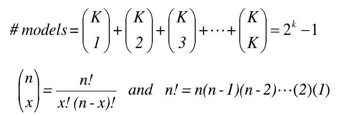
- If there are K variables (in an additive model without interaction):

Troubleshooting Regression Modeling
- Getting errors or weird results in a categorical variable with multiple categories
- Likely due to a small number of samples in some categories
- Fix: Combine categories in a way that makes sense to increase sample size in one group
- If the variable cannot be defined differently, consider excluding the variable initially and including it later on when we have less variables
- Sometimes we want to "force" a variable into a model, regardless of its significance or confounding
- This might occur when its something the readers want to know (age, sex, etc) or its the main exposure of interest
Variable Selection Methods
When no interaction exists, we have 3 primary approaches to variable selection:
- Forward
- Pick the variable most highly associated with the outcome
- Given that the variable is in the model, now pick from the remaining variables
- Continue until there are no more significant variables or all variables are in the model
- Stepwise Regression
- It is the same as the forward procedure except that at each step it looks at all variables in the model to see if they are still significantly significant (if not the variable is dropped)
- Pro:
- Speeds up process of searching through models
- More feasible than manual selection
- Cons:
- Blind analysis without thinking
- Backward methods
- Start with fully adjusted model
- Remove all variables starting with largest p-value
- Check for any confounding impact by comparing ORs before and after removal
- Stop when all remaining variables are significant or confound other variables
- Pro:
- Useful with small numbers of variables
- Cons:
- In practice it is impossible to use with a very large number of variables
Modeling with Interaction
Interaction is regarded as deviation from no interaction model, AKA multiplicative. In a multiplicative model, the order of the interaction terms can make a difference. In a hierarchical model lower order terms always come before higher order terms.
- Proceed backwards: Evaluate interaction then main effects.
- This may not be possible when possible parameters (2^k - 1) exceeds the sample size
- This can be hard to interpret and has little power for high levels of interaction.
- This procedure is applicable when there is a risk factor of interest and confounders
- Force all main effects into the model; perform stepwise regression analysis on the 2-way interactions
- It may be smart to only consider interactions having to do with the exposure of interest
- Be sure to have a hierarchical model
- Retain whatever 2-way interactions remained after step 1, perform a stepwise regression analysis on the main effects which are not part of the 2-way interactions retained
Model Selection
One can look at changes in the deviance (-2 log likelihood change)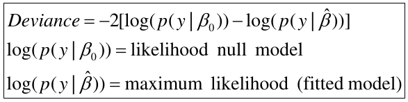
- Deviance = Residual Sum of Squares with normal data
- Problem - deviances alone do not penalize "model complexity", hence LRT is needed but only applied to nested models
- More common measures:
- AIC: Akaike's Information Criterion
- BIC, SC, SBC: Schawrtz's Bayesian Information Criterion
AIC & BIC
Both are based on likelihood. An advantage is you do not need hierarchical models to compare the AIC or BIC between models unlike -2 ln LR, the disadvantage is that there is no test or p-value that goes with comparison of models. A model with smaller values of AIC or BIC provides a better fit. When n > 7 the BIC is more conservative.
AIC and BIC can also compare non-nested models (a model where the set of independent variables in one model is not a subset of the independent variables in the other model).
The data must be the same.
Common Issues with Model Building
Collinearity occurs when independent variables in a regression model are highly correlated, or a variable can be expressed as a linear combination of other variables.
Problem: the estimate of standard errors may be inflated or deflated, so that the significance testing of the parameters becomes unreliable.
One strategy that should be used is to examine the correlations among potential independent variables, and give collinearity diagnostics. When two variables are collinear, drop one or create a new variable of both.
Risk Prediction & Model Performance
Calibration is meant to quantify how close predictions are to actual outcomes (goodness of fit)
Discrimination refers to the ability of the model to distinguish correctly the two classes of outcome
This is generally only used for dichotomous outcomes.
A model that assigns a probability of 1 to all events and 0 to nonevents would have perfect calibration and discrimination. A probability of .51 to events and .49 to nonevents would have perfect discrimination and poor calibration.
Calibration Metrics
Calibration at large: how close is the proportion of events to the mean of predicted probabilities.
Home-Lemshow Decile Approach (Logistic Regression)
- Divide the model-based predicted probabilities of size n_j
- In each decile calculate the mean of predicted probabilities p_bar_j and comare it to the observed proportion of events in that decile (r_j):

- Degrees of freedom equal to number of groups minus 2
Sensitive to small event probabilities in categories - a construct of adding 1/n_j to p_bar_j in the denominator. It is sensitive to large sample sizes.
This solution actually has serious problems; results can depend markedly on the number of groups and there's no theory to guide the choice of that number. It cannot be used to compare models.
ROC (Receiver Operating Curve)
Plots sensitivity (true positive) for different decisions and look for the best trade off between sensitivity and specificity (true negative).
- The area under the curve (AUC) is a summary measure called the c statistic;
- c is the probability that a randomly chosen subject with the event will have higher predicted probability of the event than a randomly chosen subject without the event (a measure of discrimination)
- All pairs of subjects with different outcomes are formed
- Pairs where the subject with the higher predicted value also has the higher outcome are concordant, vice versa is discordant
- > .8 is very good and < .6 is useless
Prediction, Goodness of Fit
This value can be interpreted as the "true" predictive accuracy. Methods to validate:
- Randomly split the samples into training and tesing
- Cross-validation - divide samples into k sub-samples and test on 1/k groups
- Boostrap - resample with replacement for a new sample
With any of these the analysis should be repeated many (over 100) times.
Harrell's c Survival Analysis
Calibration at large - compare how close the mean of model-based predicted probabilities at time t is to the Kaplan-Meier estimate at time t
Calibration by decile - replace rates/proportions in deciles with their Kaplan-Leier equivalents; change df to 9
- Call any two subjects comparable if we can tell which one survived longer
- Call two subjects concordant if they are comparable and their predicted prbabilities of survival agree with their observed survival times
- 'c' defined as probability of concordance given comparability
Multiple Comparisons
The significance is the probability that, in one test, a parameter is called significant when it is not (Type I error)
Multiple comparisons asks what the overall significance is when we test several hypotheses.
We can apply the Bonferroni correction (.05/n) to account for multiple comparisons.
False discovery rate - False positives among the set of rejected hypotheses, often used in studying gene expression.
Missing Data
Missing data is common in epidemiology studies, and always observed in longitudinal studies. Inadequate handling of missing data may cause bias or lead to inefficient analyses. If an estimate is incomplete, we can remove it without introduce bias. If a variable is heavily missing, it may be appropriate to remove the variable then remove all incomplete records.
There is a difference between missing and "unknown" data. Ex. someone refusing to report income on a survey would be considered missing, but an individual who has no preference between republican and democrat candidates may be considered a new category of "do not know".
Missing Data Mechanisms
The way to analyze incomplete data depends on the underlying missing data mechanisms. Ex. Is the missing data the same between males and females? Are values which are higher or lower more likely to be missing?
- Missing completely at random (MCAR): No systematic differences between the missing values and the observed values.
- Ex. Blood pressure measurements missing because of a broken tool
- In this case, the missing data mechanism is ignoreable, and missing data for the outcome can be ignored
- Missing at random (MAR): Any systemic difference between the missing values and the observed values can be explained by differences in observed data.
- Ex. Missing blood pressure measurements may be lower than those measured because younger people are more likely to be missing measurements.
- Missing not at random (MNAR): Even after the observed data are taken into account, systematic differences remain between the missing values and the observed values.
- Ex. people with hypertension missing clinic appointment because of headaches
MAR vs MCAR
- If the data are MCAR we can analyze complete cases
- If the data are MAR missing data should not be ignored
- Deterministic imputation can introduce bias/overconfidence, particularly when more than 10% of the data is missing
- Marginal imputation reduces power and bias results toward the null
- We can distinguish MCAR from MAR by observing the distribution of the indicator variable and see whether it is correlated with the observed data
Missing Data Patterns (Univariate)
Suppose we have a sample of size n, with some missing data points where: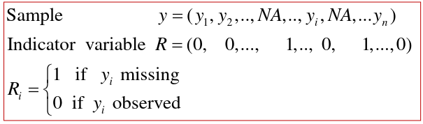
The pattern of missing data can be described via the distribution of the indicator variable R: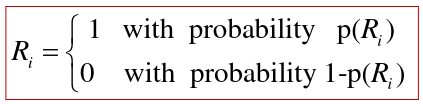
- If the probability that Ri = 1 is independent of the value yi, for any index i, the missing data pattern is ignorable. Equivalently. data are MAR
- The observed data are a random sample of complete but unobserved sample
- We can remove the data with the only effect being a decrease in power due to sample size
- If the probability that Ri = 1 is NOT independent of the value yi, for any index i, the missing data pattern is NOT ignorable, i.e. MNAR, the data are informatively missing
- The observed data does not represent a random sample of complete data.
- Missing data is not ignorable, removing it may introduce bias
Missing Data Patterns (Mutlivariate)
Assume we have a multivariate dataset with outcome Y and covariates X1-Xk
Suppose we only have missing data on Y. As in the univarite case, the patterns of missing data can be described via the distribution of the indicator variable R.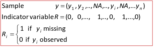
Where Ri = 1 has probability p*Ri, and Ri = 0 has probability 1-p*Ri
- If the probability that Ri = 1 is independent of the value yi, and the covariates for any index, the missing data mechanism is ignorable and the data are MCAR.
- If the probability that Ri = 1 is independent of the value yi, but is depedent the covariates for any index, the missing data mechanism is ignorable and the data are MAR. However, the observed sample may not be a random subsample of the complete one.
- If the probability that Ri = 1 is dependent of the value yi, the missing data pattern is NOT ignorable, i.e. MNAR, the data are informatively missing
Imputation
Imputation is the idea that we can fill in the missing data using either a deterministic or stochastic method or combination of both.
- Deterministic imputation
- Refers to the situation given specific values of other fields, when only one value of a field will cause the record to satisfy all of the edits, such as using the mean or median
- Stochastic (regression) imputation
- This method uses regression, it adds a random error term to the predicted value and is therefore able to reproduce the correlation of X and Y more appropriately.
Other procedures include EM algorithm, Markov Chain Monte Carlo Bayesian method, weighted methods (IPW), etc.
Multiple Imputation
To avoid the bias of the deterministic imputation, the following methods are applied:
- Imputing the missing data randomly
- Repeating the imputation many times
- Analyzing each imputed data set
- Summarizing the estimate by mean over the different sets and correct the variance
There is a paper on this by Sterne et al which explains the pitfalls and reporting procedure, but I will not go into detail here.
Other methods to fill-in missing data
- Marginal mean imputation: replace the missing y-values with the marginal mean based on the complete cases.
- This biases the data toward the null hypothesis, if the data are MCAR
- Conditional mean imputation: replace the missing y-value with the conditional mean (E(Y | X))
- This imputation biases the data toward the hypothesis of an association with the covariates
Note that to assess confounding we compute crude estimates against adjusted with the same imputed data. It is very important to use the same dataset to keep results consistent.
R Code
framdat2 <- read.table("C:/Users/liuc/Documents/BS852/BS852_Fall2021/class12/framdat2.txt",header=T, na.strings=c("."))
summary(framdat2)

# Proportion missing per variable
for(i in 1:ncol(framdat2)){
  print(names(framdat2)[i])
  print(sum(is.na(framdat2[,i]))/nrow(framdat2))
} # 6 of the variables have missing data

# Distribution of incomplete cases
num.miss <- apply(is.na(framdat2),1,sum)
table(num.miss)
length(num.miss[which(num.miss %in% c(1:6))])

MRW <- is.na(framdat2$MRW)

# Missing MRW
table(MRW)
# Missing GLI by sex
table(framdat2$SEX, MRW)/apply(table(framdat2$SEX, MRW),1,sum)

# Is missing GLI associated with sex?
summary(glm(MRW~framdat2$SEX, family=binomial(link = "logit")))

cbind(framdat2$FVC, is.na(framdat2$FVC))[1:28,]

sim.data <- read.csv("C:/Users/liuc/Documents/BS852/BS852_Fall2021/class12/sim.data.csv",header=T, na.strings=c("."))

# crude and adjusted models
summary(lm(y ~ SMOK, data=sim.data))

summary(lm(y ~ SMOK + Age + BMI + SEX, data=sim.data))

# 10% MCAR
set.seed(1234)
R <- rbinom(nrow(sim.data), p=0.10, size=1) # randomly select data to keep

mod.10mcar.crude <- lm(y ~ SMOK, data=sim.data[R==0,])

mod.10mcar.adj <- lm(y ~ SMOK + Age + BMI + SEX, data=sim.data[R==0,])

summary(mod.10mcar.crude); summary(mod.10mcar.adj)

# Marginal Mean Imputation
# 10% MCAR
set.seed(1234)
R <- rbinom(nrow(sim.data), p=0.10, size=1)

mean.obs.y <- mean(sim.data[R==0,]$y) ## complete data
sim.data$y.imputed <- sim.data$y
sim.data$y.imputed[R==1] <- mean.obs.y
boxplot(list(raw=sim.data$y, imputed=sim.data$y.imputed))

mod.imputed.crude <- lm(y.imputed ~ SMOK, data=sim.data)
summary(mod.imputed.crude)

mod.imputed.adj <- lm(y.imputed ~ SMOK+Age+BMI+SEX, data=sim.data)
summary(mod.imputed.adj)

# Conditional Mean Imputation
# 10% MCAR
set.seed(1234)
R <- rbinom(nrow(sim.data), p=0.10, size=1)

imp.model <- lm(y ~ SMOK+Age+BMI+SEX, data=sim.data[R==0,])
summary(imp.model)
imp.model$coeff
sim.data$y.imputed[R==1] <- imp.model$coeff[1]+
                                imp.model$coeff[2]*sim.data$SMOK[R==1]+
                                imp.model$coeff[3]*sim.data$Age[R==1]+
                                imp.model$coeff[4]*sim.data$BMI[R==1]+
                                imp.model$coeff[5]*sim.data$SEX[R==1]
boxplot(list(raw=sim.data$y,imputed=sim.data$y.imputed))

mod.imputed.crude <- lm(y.imputed ~ SMOK, data=sim.data);  summary(mod.imputed.crude)

mod.imputed.adj <- lm(y.imputed ~SMOK+Age+BMI+SEX, data=sim.data); summary(mod.imputed.adj)

# Distinguish MCAR from MAR
set.seed(1234)

p.miss <- c()
for (i in 1:nrow(sim.data)){
  p.miss[i] <- max(0, sim.data$Age[i]/400 + runif(n=1, min=0, max=0.02))
}

R <- c()
for (i in 1:nrow(sim.data)){
  R[i] <- rbinom(n=1, size=1, p=p.miss[i])
}

mod.mar <- glm(R ~ sim.data$Age+sim.data$BMI, family=binomial)
mod.step <- step( mod.mar, scope = R~.)
summary(mod.step)


hdl.data <- read.csv("hdl_data.csv",header=T, na.strings=c("."))

hdl.data.2 <- hdl.data[, c("SEX","BMI5","AGE5","ALC5","CHOL5","TOTFAT_C")]
summary(hdl.data.2)

summary(lm(TOTFAT_C~SEX+BMI5+AGE5+ALC5+CHOL5, data=hdl.data.2))

# Create missing data indicator for TOTFAT_C
R <- rep(0, nrow(hdl.data.2))
R[which(is.na(hdl.data.2$TOTFAT_C)==T)] <- 1

mod.mar <- glm(R ~ AGE5 + BMI5 + SEX, family = binomial, data=hdl.data.2)
step(mod.mar, scope=R~.)

library(Amelia)

set.seed(1234)
imp.data <- amelia(hdl.data.2, m=10)  ## 10 imputed datasets
summary(imp.data[[1]][[1]])

beta.bmi <- c(); se.beta <- c()
for(i in 1:10){
  mod <- lm(TOTFAT_C~SEX+BMI5+AGE5+ALC5+CHOL5, data=imp.data[[1]][[i]])
  beta.bmi <- c(beta.bmi,
  summary(mod)$coefficients[grep("BMI5", row.names(summary(mod)$coefficients)),1])
  se.beta <- c(se.beta,
  summary(mod)$coefficients[grep("BMI5", row.names(summary(mod)$coefficients)),2])}

beta.mean <- mean(beta.bmi); beta.mean
beta.var <- mean(se.beta^2) + var(beta.bmi)
beta.mean/sqrt(beta.var)

# significance based on Wald test
2*(1-pnorm(beta.mean, 0, sqrt(beta.var)))

beta.bmi <- c(); se.beta <- c()
for(i in 1:10){
    mod <- lm(TOTFAT_C~ BMI5, data=imp.data[[1]][[i]])
    beta.bmi <- c(beta.bmi,
        summary(mod)$coefficients[grep("BMI5", row.names(summary(mod)$coefficients)),1])
    se.beta <- c(se.beta,
        summary(mod)$coefficients[grep("BMI5", row.names(summary(mod)$coefficients)),2])}

beta.mean <- mean(beta.bmi); beta.mean
beta.var <- mean(se.beta^2) + var(beta.bmi)
beta.mean/sqrt(beta.var)

# # significance based on Wald test
2*(1-pnorm(beta.mean, 0, sqrt(beta.var)))