Linkage Analysis
The primary goal of linkage analysis is to determine the location (chromosome and region) of genes influencing a specific trait. We accomplish this by looking for evidence of co-inheritance of the trait with other genes or markers whose locations are known, and locating genes close to one another.
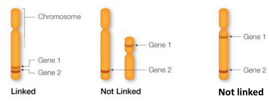
- Genes are markers that sit close together on a chromosome are called "linked" and are likely to be inherited together.
- Genes on separate chromosomes are never linked
- Genes that are far away from each other on a chromosome are likely to be separated during homologous recombination and are considered not linked
Linked Genes
Recall Mendel's 2nd Law: The Principle of Independent Assortment - Alleles of a gene pair assort independently of other gene pairs. The segregation of one pair of alleles in no way alters the segregation of another pair of alleles EXCEPT when the genes are linked on a chromosome.
A haploid genotype (haplotype) is a combination of alleles at multiple loci that are transmitted together on the same chromosome. It contains:
- The alleles present at each locus (multi-locus genotype) such as Aa Bb
- Which alleles are on the same chromosome, such as possible haplotypes Ab and aB or ab and AB
When traits are linked it means they are always inherited together. Consider the example:
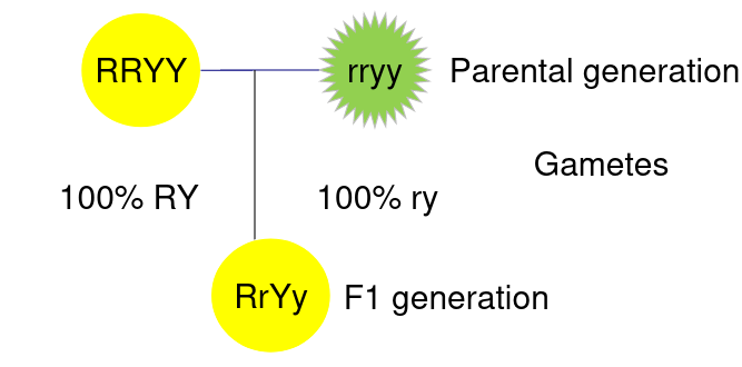
The above represents 2 different phenotytpes on a pea plant, Y is color and R is whether its round or wrinkled.
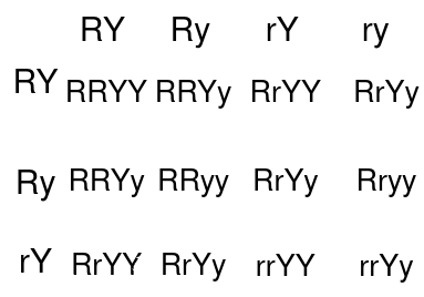
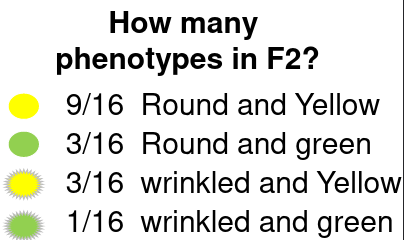
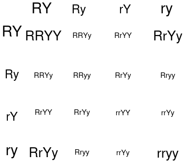
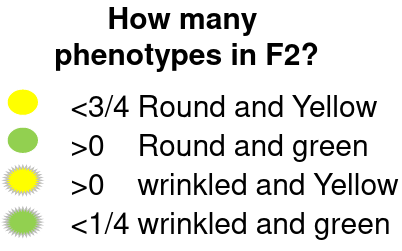
If the color and shape are unlinked then we would consider each box of a punnet square to have equal likelihood:
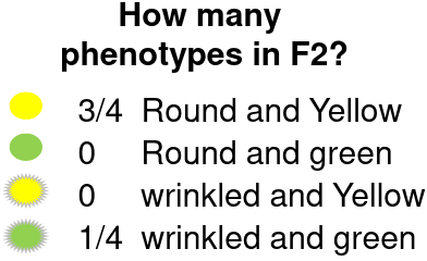
If the color and shape are completely linked then all Haploid gametes are RY or ry, that is to say R is always inherited with Y and r is always inherited with y:
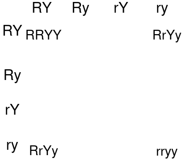
Genes can also be partially linked so the likelihood of them being paired together more likely but not guaranteed.
Recombination
Recombinant don't inherit the same chromosomes as their parents, while non-recombinant have chromosomes inherited by their parents. Proportion of recombinants gives an indication of the distance along the chromosome between the two loci; the closer they are together the less likely they are to combine.
Consider Morgan's fruit fly experiment as an example:
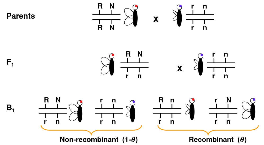
Wing length and eye color are linked. So RN and rn should always be inherited together, but we can see the recombination Rn or rN in B1 that doesn't occur in parents.
When loci are on different chromosomes, we observe recombination 50% of the time.
The line in-between the allele means they are on the same chromosome, so the alleles on the same side are inherited together.
Overview of Recombination
The recombination fraction (theta) is the probability of recombination (i.e. the probability of an odd number of crossovers) between two loci. The further apart they are, the more likely they are to recombine and vice versa.
- 𝜃 = 0 if:
- The genetic marker is the polymorphism causing the disease
- The marker is so close to the disease mutation that recombination can never occur
- 𝜃 = .5 if:
- There is a 50% chance that alleles at the two loci are inherited together. This happens when the two loci are
- Very far apart on a chromosome
- Located on two different chromosome
- There is a 50% chance that alleles at the two loci are inherited together. This happens when the two loci are
Linkage Analysis
Linkage analysis estimates the genetic distance between genetic markers or between genetic markers and a trait locus with recombination. This allows us to know where a trait locus is in the genome if we know:
- The genetic distance between a disease locus and a marker
- The location of the marker on the genome.
To perform a linkage analysis, estimate the recombination fraction between the disease locus and a marker locus and test:
H0: 𝜃 = 1/2 -> not linked i.e segregating independently
H1: 𝜃 < 1/2 -> linked, i.e. close together on the same chromosome
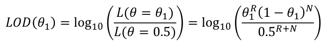
The most common test of linkage is Logarithm of the Odds (LOD):
LOD Score = log base 10 of the likelihood ratio = log10(L(𝜃=𝜃1)/L(𝜃=.5))
This is a transformation of the usual likelihood ratio test. The probability of observing R recombinants and N non-recombinants, where the recombination fraction is 𝜃, the binomial is as follows:
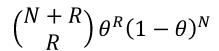
So the likelihood is:
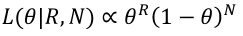
We can ignore the constant because we will be working with a ratio of likelihoods and the constant cancels.
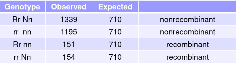
When we know the exact number of recombinants and non-recombinants:
The MLE of 𝜃 is 𝜃_hat = R/(R+N) which is the value of 𝜃 that maximizes the LOD score and likelihood function.
- LOD score > 3 -> linkage
- LOD score (for a particular q value) < -2 -> no linkage
- When the LOD scores is between 3 and -2, results are inconclusive. We might want to obtain additional individuals, additional families or utilize additional markers
Factors Influencing Linkage Analysis
- Penetrance - the probability of expressing the disease given a specific genotype.
- Age dependent penetrance is also common in some diseases, such as Huntingtons.
- Ex. reduced penetrance could be P(Disease | DD or Dd) < 1.0 for Autosomal Dominant
- Age dependent penetrance is also common in some diseases, such as Huntingtons.
- Genetic Heterogeneity - multiple genes which mutations cause the same phenotype
- When heterogenetiy exists LOD score over families may not show evidence of linkage, but significant linkage may occur within a subset
- Ex. there are 7 genes identified for fmilial Parkingson's disease; some dominant, some recessive.
Overview of Linkage Analysis
Parametric linkage analysis assesses linkage between a marker and a locus
- Need to specify a model for the inheritance of the disease
- Need to specify risk allele frequency
- Need to specify penetrances
Advantages
- Most powerful approach when the model is correctly specified
- It utilizes every family member's phenotypic and genotypic information
- It provides a statistical test for linkage and for genetic heterogeneity
Disadvantages
- Poor power if the genetic model is misspecified
- Unaffected individuals may provide little information if penetrance is low
- Can be difficult to recruit large families
Multi-point Linkage Analysis
Multi-point analysis incorporates multiple markers into the likelihood computation. It computes the likelihood that a disease is located at a certain position on a chromosome. The null hypothesis is that the disease locus is not on the chromosome. It has more information and thus is more powerful.
Affected Relative Pairs
Based on sets of affected pairs, no need to specify a model. This is a non-parametric tests of linkage analysis. Easier to collect but need a larger sample.
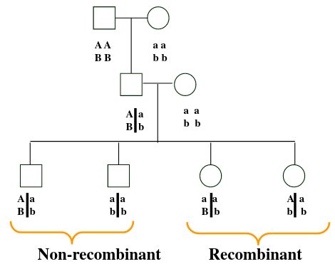
Alleles that are copies of the same allele from a common ancestor are called "identical-by-descent" or IBD for short. IBS is "Identity-by-state". All IBD are IBS but the opposite is not true.
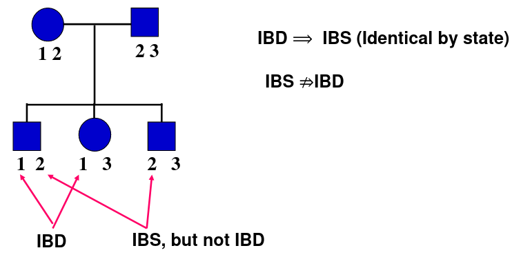
For the bottom rightmost "3" in the example definitely comes from the father, so it is shared IBD.
The logic behind this test is that if an allele is "causing" a disease, and the disease is not common, two affected relatives will most probably share the allele IBD. This means the surrounding region will most probably be IBD, and we can look for regions which are more likely to hold the disease locus.
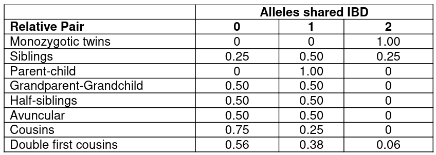
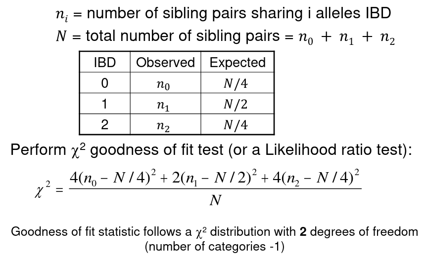
Consider the below chart with the expected frequency of relative pairs showing sharing 0,1, or 2 alleles IBD under no linkage:
The process of linkage analysis through affected relative pairs is as follows:
- Collect a sample of pairs of affected relatives
- Genotype some markers and estimate IBD
- At multiple locations across the genome test whether the pairs share more alleles IBD than would be expected by chance.
Tests for affected sibling pairs:
- Goodness of Fit
- Mean Sharing Test (not covered here)
- Nonparamtric Linkage Analysis Score Test (NPL), best for affected general relatives (not covered here)
Goodness of Fit
Linkage Measured By LOD Score
LOD Score = log_10(Likelihood Ratio)
Likelihood Ratio Test (LRT) = 2 * ln(Likelihood Ratio) ~ chi2
Therefor: chi2 = 2 * ln(10) * log_10(likelihood ratio) = 4.6 * LOD Score
LOD Score = chi2 test value / 4.6, with 1 df
LOD score ~ z2 / 4.6 or t2 / 4.6
Quantitative Trait Locus Mapping
Relatives who have similar trait values should have higher than expected levels of sharing genetic material near the genes that influence those traits (a greater IBD).
The Haseman-Elston (HE) was the first approach to QTL in humans.
- Let Y_1j and Y_2j be the phenotypes of siblings 1 and 2 of the jth subpair
- Y_j^D = (Y_1j - Y_2j)^2 -> the difference in sib phenotypes
- pi_j the proportion of alleles shared IBD by the jth sibpair at the marker of interest. Could be 0, .5, or 1 when IBD is known with certainty. Otherwise it is a range from 0 to 1.
- To test for linkage perform the linear regression of:
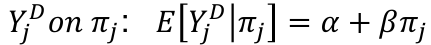
It can be proven that:
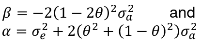
Where sigma_squared_a is the genetic variance explained by the locus and sigma_squared_e is the envoirnmental variance of the trait.
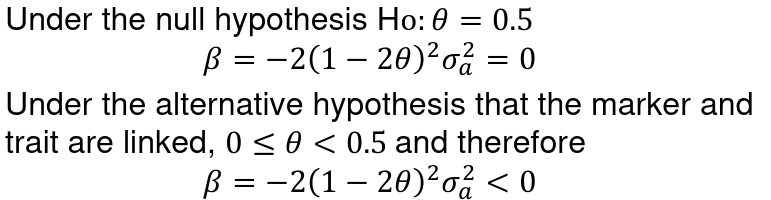
A negative slope implies linkage, as relatives with similar trait values have small squared differences and high IBD sharing