Statistical Genetics

• Genetics and Inheritance
• Linkage Analysis
• Assessing the Genetic Component of a Phenotype
• Population Genetics
• Association Testing in Unrelated Individuals
• Multiple Comparisons and Evaluating Significance
• Association Testing in Related Individuals
• Haplotypes and Imputation
• Power and Sample Size Calculations for Association Studies
• Sequencing Data and Analysis of Rare Variants
• Interactions in Genetic Assocation Analysis
• Meta Analysis

Genetics and Inheritance

Gregor Mendel was an Austrian Monk in the late 1800s who experimented with pea plants to find trait inheritance patterns in successive generations.

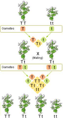
Mendel's Laws

1. Principle of Segregation - Two alleles of a homologous pair of chromosomes separate (segregate) during gamete formation such that each gamete receives only one allele
2. Principle of Independent Assortment - Alleles of a gene pair assort independently of other gene pairs. The segregation of one pair of alleles in no way alters the segregation of another pair of alleles*

*This law is not always true, when genes are linked on a chromosome, explained later

Terminology

Homozygous - An individual who has two copies of the same allele at a locus

Heterozyous - An individual who has two different alleles at the same locus

Dominant alleles only needs one copy to show the phenotype

Recessive alleles need two copies of the allele to show the phenotype

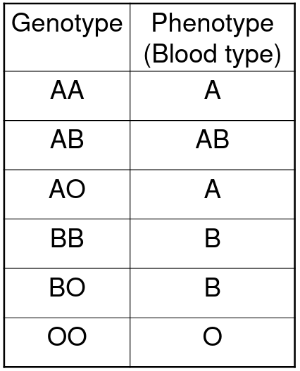
Co-dominance means the phenotype for the heterozygote is different from either homozygote

Example - Blood types A and B are co-dominant to each other, but dominant to type O:

Gene inheritance only happens during Meiosis, not mitosis (although mutations can happen in both). If you have genes close to each other, they are more likely to be inherited together, which is why Mandel's second law does not always hold.

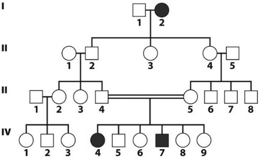
Pedigree Drawing

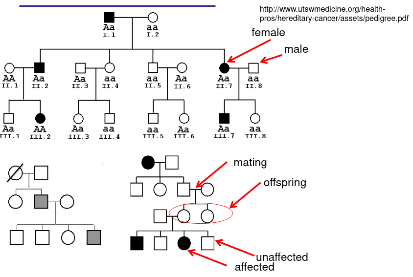
Diagonal line mean the person is deceased. Filled in represents individuals effected by a certain condition of interest, a half filled in shape represents a "carrier" of the condition who does not express it.

• Carrier - Individuals who carry a gene of interest
  
• Obligate carrier - one who must be a carrier due to observed affected in pedigree

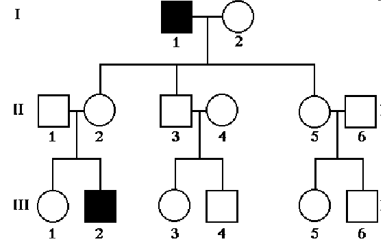
Mendelian Diseases

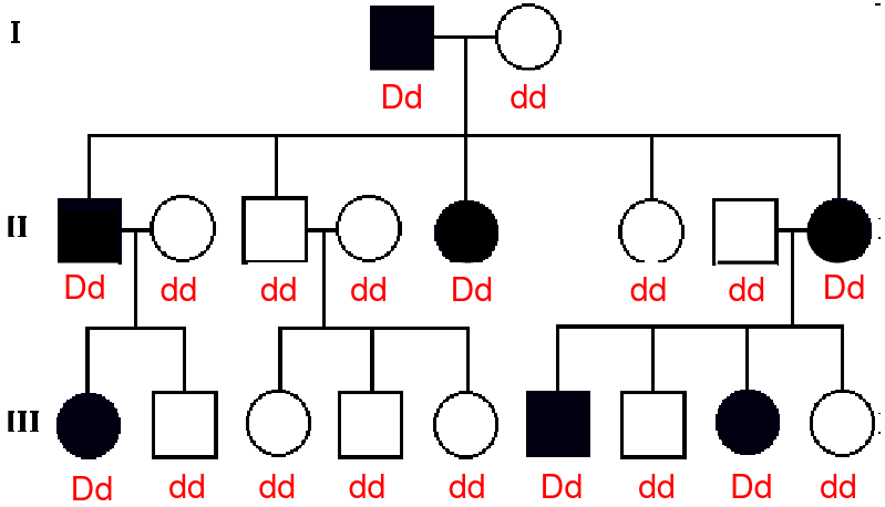
Mendelian diseases are disorders caused by a mutation in a single gene. Follow a specific form of inheritance, the most common:

• Autosomal dominant- needs a single copy of the mutated disease gene to express the disease
  
  • Vertical transmission of the disease phenotype
  • Lack of skipped generations
  • Roughly equal numbers of affected males and females
  • Father-son transmission may be observed
  • Roughly half of the offspring of an affected parent will be effected

• Autosomal recessive - Two copies of the mutated gene required to express disease.
  • Clustering of the disease phenotype in siblings
  • The disease is not seen in parents
  • Equal numbers of affected males and females
  • Consanguinity (marriage between related individuals) may be present

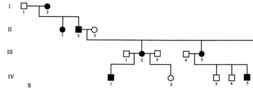
• X-linked recessive
  • Never passed from father to son
  • Males are much more likely to be affected
  • Affected males get the disease from their unaffected carrier mothers; all of their daughters are obligate carriers
  • Sons of carrier females have a 50% chance of receiving the mutant alleles
  • Typically passed from an affected grandfather to 50% of his grandsons through daughters

• X-linked dominant
  • Daughters of affected males will inherit the disease from their fathers
  • Sons of the affected males cannot inherit the disease from their father (they receive Y chromosome from father)
  • Sons and daughters of affected heterozygous mothers have 50% chance of inheriting the disease
  • On average, twice as many affected females compared to affected males
  • Males are often more severely affected
  • May be associated with miscarriage or lethality in males

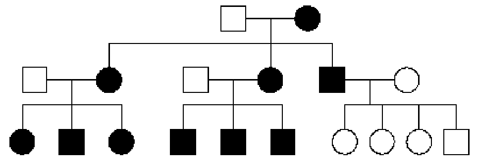
• Mitochondrial inheritance
  • All children of affected females are affected
  • None of the children of affected males are affected
  • There are relatively few human diseases caused by mitochondrial mutations

Any trait that does not follow a Mendelian pattern is a complex genetic trait

Storing Family Data

There are really no standards for storing genetic data, everyone has their own way of representing it.

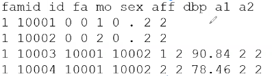
Here is a typical representation of a pedigree data set. 2 indicates something is present and 1 indicates it is not. Be prepared to draw a pedigree chart from something like the above.

a1 and a2 are the alleles being studied and aff is if the indicivdual is affected by the trait. We might represent the allele pair as 11, 12, 22 or 1/1, 1/2, 2/2, etc.

SNP (SNV) "single nucleotide polymorphism/variant" genotypes may be:

• Numbers (1 or 2 to indicate the two possible alleles)
• Letters (A, T, C, G to indicate bases)
• Numbers (1, 2, 3, 4) to indicate the above bases

Microsatellites may be recorded as:

• Allele lengths (number of base pairs) or number of repeats
• Consecutive numbers from 1- number of alleles which may or may not correspond to allele size

Sometimes phenotype may be complex, where it is than affected/unaffected, in which case it is usually store separately from the genetic data.

Useful Summary Information of Genetic Data

• Number of individuals genotyped
• Genotype frequencies
• Allele frequencies
• Proportion of individuals with missing markers
• Proportion of missing markers for an individual
• Number of families and number genotyped in each family, if using family data
• For quantitative traits (blood pressure, cholesterol, etc) can use averages and ranges

Linkage Analysis

The primary goal of linkage analysis is to determine the location (chromosome and region) of genes influencing a specific trait. We accomplish this by looking for evidence of co-inheritance of the trait with other genes or markers whose locations are known, and locating genes close to one another.

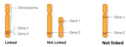
• Genes are markers that sit close together on a chromosome are called "linked" and are likely to be inherited together.
• Genes on separate chromosomes are never linked
• Genes that are far away from each other on a chromosome are likely to be separated during homologous recombination and are considered not linked

Linked Genes

Recall Mendel's 2nd Law: The Principle of Independent Assortment - Alleles of a gene pair assort independently of other gene pairs. The segregation of one pair of alleles in no way alters the segregation of another pair of alleles EXCEPT when the genes are linked on a chromosome.

A haploid genotype (haplotype) is a combination of alleles at multiple loci that are transmitted together on the same chromosome. It contains:

1.  The alleles present at each locus (multi-locus genotype) such as Aa Bb
   
2. Which alleles are on the same chromosome, such as possible haplotypes Ab and aB or ab and AB
   

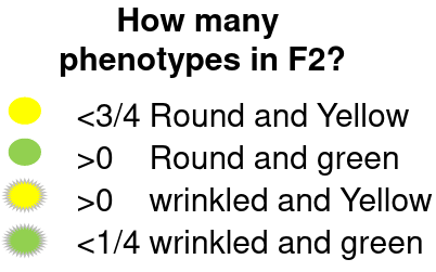
When traits are linked it means they are always inherited together. Consider the example:

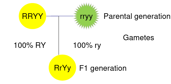
The above represents 2 different phenotytpes on a pea plant, Y is color and R is whether its round or wrinkled.

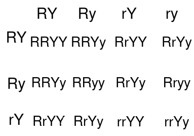
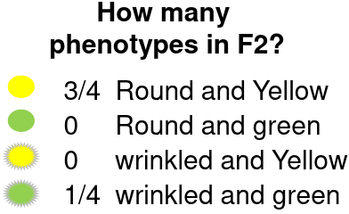
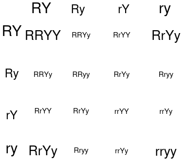
If the color and shape are unlinked then we would consider each box of a punnet square to have equal likelihood:

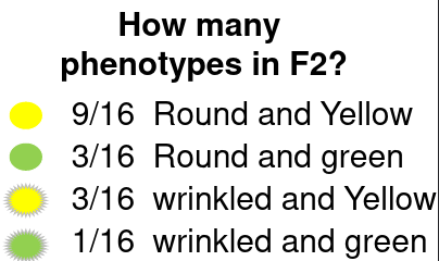
If the color and shape are completely linked then all Haploid gametes are RY or ry, that is to say R is always inherited with Y and r is always inherited with y:

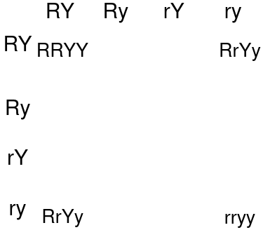
Genes can also be partially linked so the likelihood of them being paired together more likely but not guaranteed.

Recombination

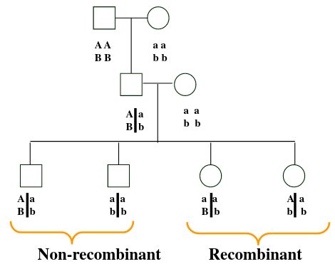
Recombinant don't inherit the same chromosomes as their parents, while non-recombinant have chromosomes inherited by their parents. Proportion of recombinants gives an indication of the distance along the chromosome between the two loci; the closer they are together the less likely they are to combine.

Consider Morgan's fruit fly experiment as an example:

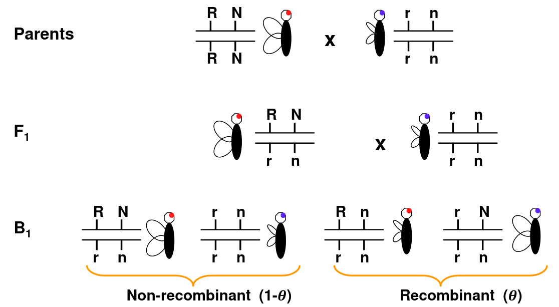
Wing length and eye color are linked. So RN and rn should always be inherited together, but we can see the recombination Rn or rN in B1 that doesn't occur in parents.

When loci are on different chromosomes, we observe recombination 50% of the time.

The line in-between the allele means they are on the same chromosome, so the alleles on the same side are inherited together.

Overview of Recombination

The recombination fraction (theta) is the probability of recombination (i.e. the probability of an odd number of crossovers) between two loci. The further apart they are, the more likely they are to recombine and vice versa.

𝜃 is related to how closely "linked" the two loci are, and ranges from 0 to .5

• 𝜃 = 0 if:
  • The genetic marker is the polymorphism causing the disease
  • The marker is so close to the disease mutation that recombination can never occur
• 𝜃 = .5 if:
  
  • There is a 50% chance that alleles at the two loci are inherited together. This happens when the two loci are
    • Very far apart on a chromosome
    • Located on two different chromosome

Linkage Analysis

Linkage analysis estimates the genetic distance between genetic markers or between genetic markers and a trait locus with recombination. This allows us to know where a trait locus is in the genome if we know:

1. The genetic distance between a disease locus and a marker 
2. The location of the marker on the genome.

To perform a linkage analysis, estimate the recombination fraction between the disease locus and a marker locus and test:

H0: 𝜃 = 1/2 -> not linked i.e segregating independently

H1: 𝜃 < 1/2 -> linked, i.e. close together on the same chromosome

The most common test of linkage is Logarithm of the Odds (LOD):

LOD Score = log base 10 of the likelihood ratio = log₁₀(L(𝜃=𝜃₁)/L(𝜃=.5))

This is a transformation of the usual likelihood ratio test. The probability of observing R recombinants and N non-recombinants, where the recombination fraction is 𝜃, the binomial is as follows:

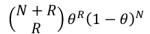
So the likelihood is:

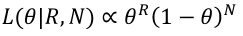
We can ignore the constant because we will be working with a ratio of likelihoods and the constant cancels.

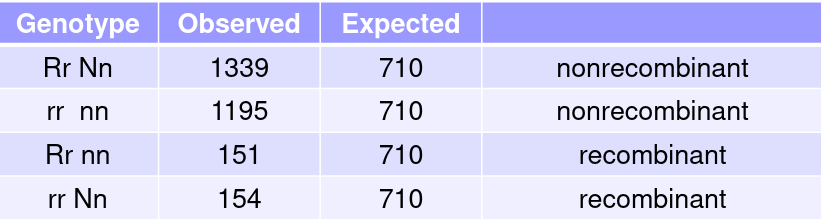
When we know the exact number of recombinants and non-recombinants:

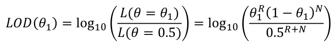
The MLE of 𝜃 is 𝜃_hat = R/(R+N) which is the value of 𝜃 that maximizes the LOD score and likelihood function.

• LOD score > 3 ->  linkage
• LOD score (for a particular q value) <  -2  ->  no linkage
• When the LOD scores is between 3 and -2, results are inconclusive. We might want to obtain additional individuals, additional families or utilize additional markers

Factors Influencing Linkage Analysis

• Penetrance - the probability of expressing the disease given a specific genotype.
  • Age dependent penetrance is also common in some diseases, such as Huntingtons.
    
  • Ex. reduced penetrance could be P(Disease | DD or Dd) < 1.0 for Autosomal Dominant
• Genetic Heterogeneity - multiple genes which mutations cause the same phenotype
  • When heterogenetiy exists LOD score over families may not show evidence of linkage, but significant linkage may occur within a subset
  • Ex. there are 7 genes identified for fmilial Parkingson's disease; some dominant, some recessive.

Overview of Linkage Analysis

Parametric linkage analysis assesses linkage between a marker and a locus

• Need to specify a model for the inheritance of the disease
• Need to specify risk allele frequency
• Need to specify penetrances

Advantages

• Most powerful approach when the model is correctly specified
• It utilizes every family member's phenotypic and genotypic information
• It provides a statistical test for linkage and for genetic heterogeneity

Disadvantages

• Poor power if the genetic model is misspecified
• Unaffected individuals may provide little information if penetrance is low
• Can be difficult to recruit large families

Multi-point Linkage Analysis

Multi-point analysis incorporates multiple markers into the likelihood computation. It computes the likelihood that a disease is located at a certain position on a chromosome. The null hypothesis is that the disease locus is not on the chromosome. It has more information and thus is more powerful.

Affected Relative Pairs

Based on sets of affected pairs, no need to specify a model. This is a non-parametric tests of linkage analysis. Easier to collect but need a larger sample.

Alleles that are copies of the same allele from a common ancestor are called "identical-by-descent" or IBD for short. IBS is "Identity-by-state". All IBD are IBS but the opposite is not true.

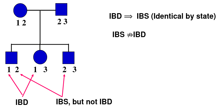
For the bottom rightmost "3" in the example definitely comes from the father, so it is shared IBD.

The logic behind this test is that if an allele is "causing" a disease, and the disease is not common, two affected relatives will most probably share the allele IBD. This means the surrounding region will most probably be IBD, and we can look for regions which are more likely to hold the disease locus.

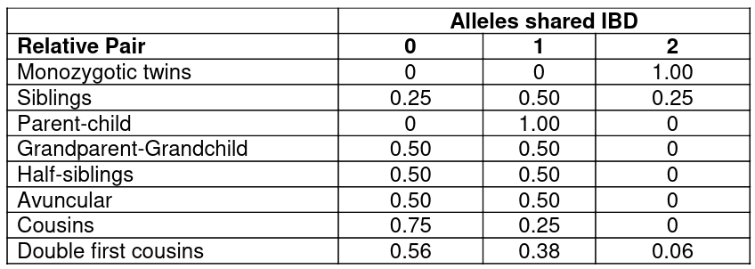
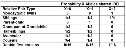
Consider the below chart with the expected frequency of relative pairs showing sharing 0,1, or 2 alleles IBD under no linkage:

Twins always share their alleles. Children always inherit 1 allele IBD with their parents, making the relationship useless for linkage analysis. Siblings can give the most information.

The process of linkage analysis through affected relative pairs is as follows:

1. Collect a sample of pairs of affected relatives
2. Genotype some markers and estimate IBD
3. At multiple locations across the genome test whether the pairs share more alleles IBD than would be expected by chance.

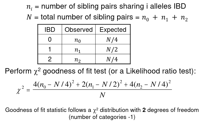
Tests for affected sibling pairs:

• Goodness of Fit
• Mean Sharing Test (not covered here)
• Nonparamtric Linkage Analysis Score Test (NPL), best for affected general relatives (not covered here)

Goodness of Fit

Linkage Measured By LOD Score

LOD Score = log_10(Likelihood Ratio)

Likelihood Ratio Test (LRT) = 2 * ln(Likelihood Ratio) ~ chi²

Therefor: chi² = 2 * ln(10) * log_10(likelihood ratio) = 4.6 * LOD Score

LOD Score  = chi² test value / 4.6, with 1 df

LOD score  ~ z² / 4.6 or t² / 4.6

Quantitative Trait Locus Mapping

Relatives who have similar trait values should have higher than expected levels of sharing genetic material near the genes that influence those traits (a greater IBD).

The Haseman-Elston (HE) was the first approach to QTL in humans.

• Let Y_1j and Y_2j be the phenotypes of siblings 1 and 2 of the jth subpair
• Y_j^D = (Y_1j - Y_2j)^2 -> the difference in sib phenotypes
• pi_j the proportion of alleles shared IBD by the jth sibpair at the marker of interest. Could be 0, .5, or 1 when IBD is known with certainty. Otherwise it is a range from 0 to 1.
• To test for linkage perform the linear regression of:

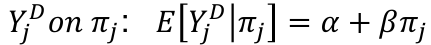
It can be proven that:

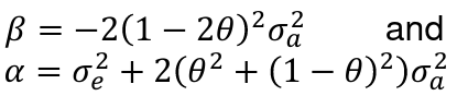
Where sigma_squared_a is the genetic variance explained by the locus and sigma_squared_e is the envoirnmental variance of the trait.

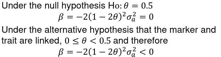
A negative slope implies linkage, as relatives with similar trait values have small squared differences and high IBD sharing

Assessing the Genetic Component of a Phenotype

A phenotype is the appearance of an individual, which results from the interaction of the person's genetic makeup and their environment. Phenotypes can be categorical or numerical. If we are interested in the genetic component of a trait  there are different methods we can use for analysis.

We define a trait for analysis, determine what we are interested in studying, and then the methods that need to be used. For example, if we want to know how BMI is linked to gene effects we would need to consider other factors such as age, sex, smoking, etc. Thus, a Multiple Linear Regression might be appropriate, were we can measure the variability of each factor.

Variance of Phenotypic Traits

𝜎²_T = The observed (phenotypic) variability of a trait
𝜎²_T = 𝜎²_G + 𝜎²_E = The phenotypic variability can be partitioned in to variability due to genetic and environmental effects
𝜎²_G = 𝜎²_A + 𝜎²_D = The genetic component can be further partitioned into additive and dominance genetic variance

We can write a model for the trait as:  
T = (A + D) + E = G + E

Assumptions of this model:

• Genetic and environmental factors are uncorrelated
• Standard deviation of trait is the same for all individuals

Additive and Dominance Components

Consider a frequency distribution of trait values for two alleles B and b, where B creates a high trait value and b creates a low trait value on a continuous scale which is shifted so that the midpoint between the mean of BB (+a) and bb (-a) is 0:

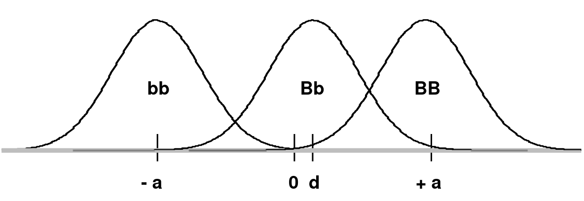
d is the mean of the Bb group

In an additive model d = 0 (no dominance; dominance variance = 0)
In a recessive model: d = -a    (Bb would overlap the bb distribution)
In a dominant model d = +a   (Bb would overlap the BB distribution)

The degree of dominance can be defined as d/a

Heritability

The heritability of a trait is the proportion of total phenotypic variance that is due to genetic effects.

Heritability can be defined as:

h²    =    𝜎²_G /  𝜎²_T     =   ( 𝜎²_A + 𝜎²_D ) / ( 𝜎²_A + 𝜎²_D + 𝜎²_E )

The above formula is also called Broad sense hertiability. Narrow sense heritability (just the additive component): 

h_n²    =  𝜎²_A  / 𝜎²_T

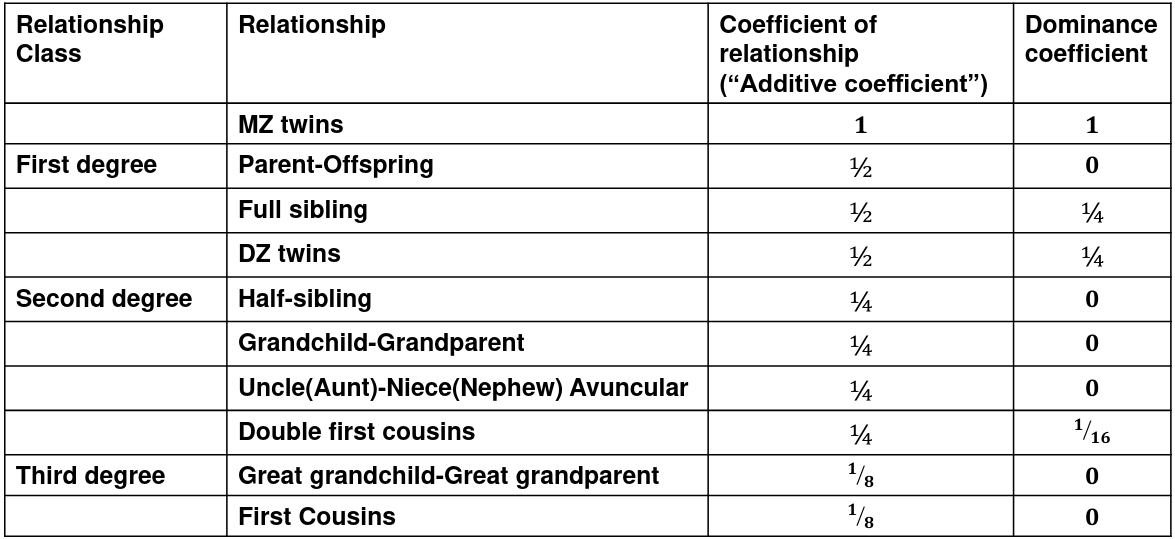
We use the expected resemblance among relatives to estimate h². It is a function of covariance between relatives and coefficient of relationship (AKA "Additive coefficient")

The additive coefficient of a relationship C is the expected proportion of alleles shared IBD by a relative pair, defined as:

C = 2^-R, where R is the degree of relationship

• R = 0: MZ twins -> C = 1
• R = 1: 1st degree relationship; sib, parent-offspring -> C = 1/2
• R = 2: 2nd degree relatives: half-sibs, grandparent-grandchild, avuncular
• R = 3: 1st cousins

Recall sharing a allele Identical-By-Descent means relatives who share the exact same copy of an allele by inheritance.

The additive coefficient is expected proportion of alleles shared IBD by the pair, so we can also define it as

p(x) = x/2 = the proportion of shared alleles

For example, the parent child relationship would have a additive coefficient of 0*(0/2) + 1*(1/2) + 0*(2/2) = 1/2

The kinship coefficient is the probability that a randomly selected pair of alleles from a individual is IBD. It is always half of the coefficient of relationship.

Estimating Heritability

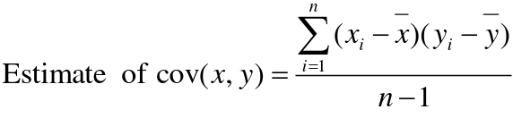
Using Co-variance

Recall the properties of covariance:

• Cov(X,Y) = Cov(Y,X)
• Cov(X, X) = var(X)
• Cov(X + Y, Z) = Cov(X, Z) + Cov(Y, Z)
• Cov(cX, Y) = c*Cov(X,  Y); where c is some constant
• The unit of covariance is xy
• Positive covariance: Value of x tends to be high when value of y is high
• Negative covariance: Value of x tends to be high when value of y is low

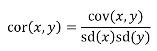
A standardized measure of covariance is correlation which is a scale of -1 to 1

We can use the properties of covariance to determine the covariance between quantitative measure on a parent and an offspring. This folows the same T = (A + D) + E = G + E concept as above:

Cov(Parents, Offsrping) = Cov (A_p + D_p + E_p, A_o + D_o + E_o)

In this example, we can break this down into:

• Cov (A_p, A_o) = Additive covariance, offspring always inherits exactly 1 allele from parent so = (1/2)𝜎²_A 
  
• Cov (E_p, E_o),  covariance of environmental component between parent and offspring is assumed to be 0
  
• Cov (D_p, D_o) = Since offspring do not inherit pairs of alleles the dominance environmental component is also 0
  
• The cross terms, Cov(A, D) and etc. which we assume to be 0

Note: This only works if the assumptions of independence is true and standard deviation is the same for all individuals.

Since we are assuming standard deviation is the same across generations we can write hieritability between parent and offspring as a product of correlation:

h_n² =  𝜎²_A  / 𝜎²_T = 2 * Cov(parent, offspring) / SD(parent)*SD(child) = 2 * Cor(parent, offspring)

Thus, we can estimate narrow-sense heritability using 2 times the observed correlation between parents and offspring.

Using Linear Regression

Alternatively, we can use the linear regression coefficient to estimate heritability. Where Y is offspring and X is parent:

𝑌 = 𝛼 + 𝛽𝑋 + 𝐸

 𝛽_hat ~ cor(X, Y) x SD(Y)/SD(X)

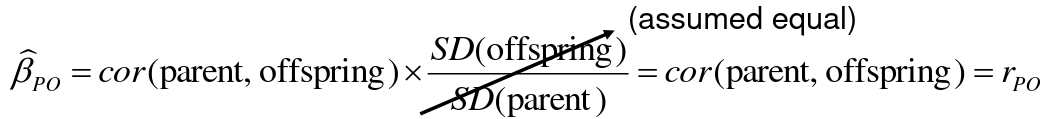
h_n² = 2*r_PO = 2*𝛽_hat_PO

Note that the estimate obtained from beta may differ from the estimate obtained from r if the standard deviations of parents and offspring are not equal.

If both parents are available we can regress the offspring value of the mean parental phenotype value:

h² = 𝛽_hat_MO  

Beta estimates heritability directly in the average parent version. I'm not going show the math here, but know this is in part due to SD(average parent) = SD(parent) / sqrt(2)

Example with Sibling Pairs

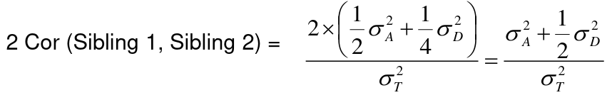
Looking at the relationship table above in the siblings row: additive coefficient is 1/2 and dominance coefficient 1/4. If data is available on N sibling pairs only:

Cov(Sibling 1. Sibling 2) = (1 / 2) 𝜎²_A + (1 / 4) 𝜎²_D 

If 𝜎²_D   = 0, 2 times the intraclass correlation (ICC) is an estimate of heritability: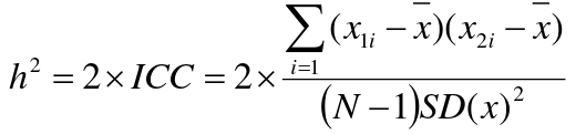
Where x and SD(x) are computed combining data on all siblings.

If 𝜎²_D  does not equal 0, this estimate is between the narrow and broad heritability because:

Intraclass Correlation Vs. Pearson (Product-Moment) Correlation

When pairs consist of individuals of two different classes (grandparent-grandchild, parent-offspring) we call this pairwise correlation and we can use a simple Pearson correlation coefficient:

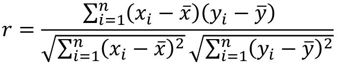
But when the pairs have no obvious order (siblings or cousins), the intraclass correlation is used:

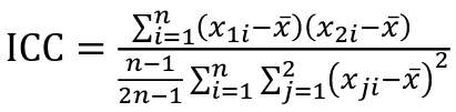
where n is the number of pairs and x_bar is the mean value across all individuals

The main difference between the product-moment correlation and ICC:

• ICC: SD in the denominator is pooled across individuals
  
• Pearson: SD for the two types of relatives are computed separately

ICC can be extended to sets of 3 or more. The formula for ICC is:

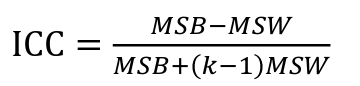
k = number of siblings per sibship
MSB = Mean Square Between (model)
MSW = Mean Square Within (error)
If the sibships are of unequal size using the average sibship size will provide an approximate h² estimate

h² = 2 * ICC

Twin Studies

Monozygotic twins are genetically identical and dizygotic twins are genetic the same as a full sibling, sharing half their genes on average. A common estimate of heritability in studies with both mono and dizygotic twins can estimate it as:

h² = 2 * (ICC_MZ - ICC_DZ)

If 𝜎²_D  does not equal 0, this estimate is greater than both the narrow and broad heritability because:

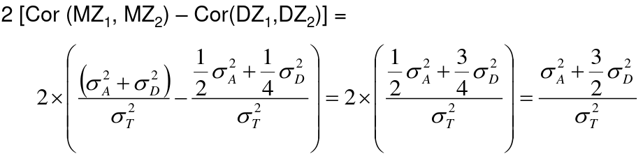
This is in part because we cannot assume there is no shared environmental variance in siblings and especially twins.

Notes on Estimating Heritability

• We can obtain different estimates using different subsets of data
• Differences in estimates may be due to "sampling variation"
• If the dominance variance is not 0, some differences may be expected
  • Siblings and twins incorporate dominance variance; parent-offspring do not
• Siblings and twins tend to share environment/exposure factors
• We may get smaller estimates with pairs that are more similar (Age, weight, etc)
• Precision of heritability estimates depends on the SE of the correlation coefficient or regression coefficient used for the estimation
• Large sample sizes are needed to get precises measures of heritability
• Heritability is a ratio of variances, not an average
• Law of large numbers does not necessarily apply here, heritability does not necessarily follow a normal distribution
• Maximum likelihood approach can be used to estimate  𝜎²_{T ,} 𝜎²_A, and 𝜎²_D -- and can also estimate shared environments when we are not assuming it to be 0 

We can estimate the linear mixed effects (variance component model):

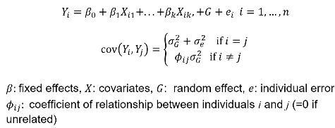
In which case we would estimate heritability as 𝜎²_G and test H0: 𝜎²_G  = 0

Heritability Summary

• Heritability is a population parameter, defined as the proportion of trait variance explained by additive genetic factors
  • Estimates of h² are usually based on resemblance between relatives
  • Highly heritable -> close relatives should be more correlated 
• Heritability may differ by population
  • h² depends on both 𝜎²_T  and 𝜎²_A
• h² estimates using close and distant relatives should be similar
  • Estimates bases on twins, sibs and cousin pairs estimate the same population parameter (unless there is dominance variance)
• If a trait is not heritable (h² = 0), we do not expect close relatives to be more correlated than distance relatives
• Heritability is generally computed for quantitative traits with analysis of variance, but can also be estimated for discrete traits
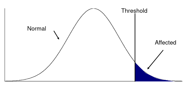
  • Liability, or predisposition to disease, is measured on a quantitative scale
  • Threshold model: trait present if liability to disease exceeds a certain threshold
  • Heritability measures the liability between relatives
  • There is specialized software for calculating this
  • Referred to as the "latent variable" model, we can observe whether an individual has cross the threshold

Recurrence Risk Ratio

Recurrence risk ratio assess familial aggregation of dichotomous traits (diseases).  𝜆_𝑅 denotes relative risk with a subscript indicating the specific type of relative examined.

A proband is a subject selected for a study due to disease status. In familial disease studies, it is the affected subject that brought the family into the study

𝜆_𝑅 = 𝐾_𝑅/𝐾
𝐾_𝑅 = P(disease | relative of type R is affected) =  the proportion (prevalence) of relatives of affected probands that are affect with disease
K = the proportion of affected individuals in the general population

General rule:

• If a trait is generic 𝜆_𝑅 should decrease as degree of relationship increases
• Differences in shared environment may lead to differences in 𝜆_𝑅 for different relative types of the same degree
• 𝜆_𝑅 may be greater than 1 when the trait does not have a genetic component due to a shared enviornment
  

Population Genetics

Genotype and Allele Frequency Estimation is the first step in studying a polymorphism. Used for family data and independent individuals in a population. We can use a subset of individuals who are independent and count alleles, or use the maximum likelihood methods to take all genotypes into account for pedigree data.

Consider the following example of allele frequency estimation: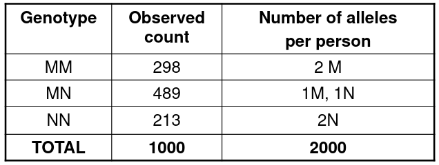
We can take the frequency of each allele by the observed proportions:
    p_M = (2*298 + 489)/(2*1000)
    p_N = 1 - pM

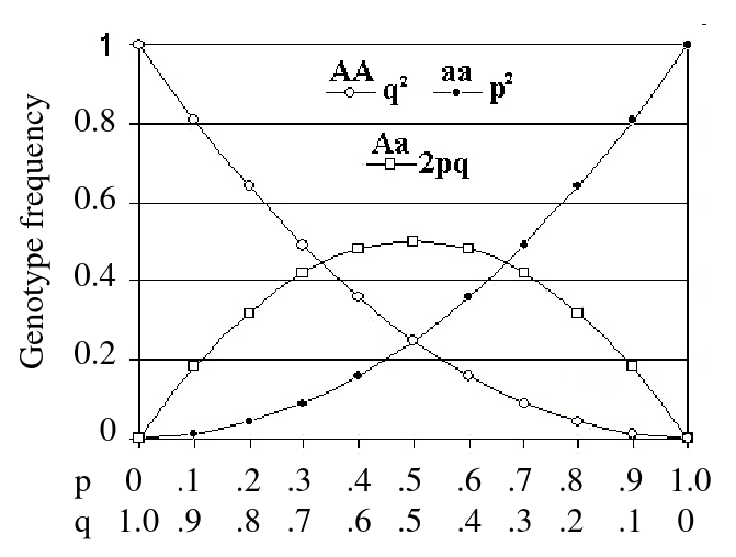
Hardy-Weinberg Law

Describes how we expect allele frequencies and phenotype frequencies to be related in a population.

1. For a large, random-mating population, in the absence of forces that change allele frequencies, the allele and genotype frequencies remain constant from one generation to the next
2. After one generation of random mating, for an autosomal locus with alleles 1 and 2 (frequencies p and q = 1 - p), the relative frequencies of the genotypes 11, 12, and 22 are:
        p², 2pqm q²

Assumptions

• Random mating with respect to genotype
  • No assortative mating
  • No population structure
• No selection, mutation, or migration
• Discrete generations
• Infinite population size
• Autosomal locus

Given two alleles with 1 and 2, there are 6 possible parent mating types: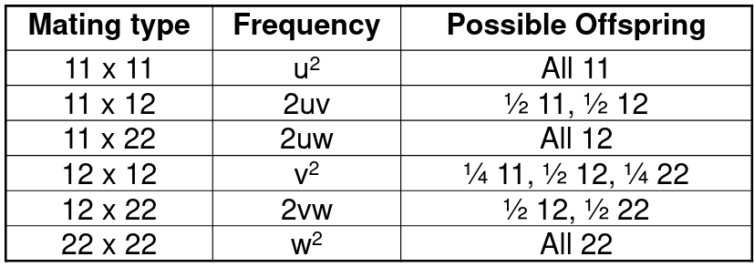

So the frequency of allele 1 in the offspring would be:
    P(11) + ½P(12) = (u+v/2)2 + (u+v/2)(v/2+w) = (u+v/2)(u+v+w) = u+v/2

Similarly, the frequency of allele 2 is: w + v/2

Forces that change allele or genotype frequency (invalidate HW law)

• Mutation
• Migration
• Selection
  • Deleterious mutations tend to be rare if there is selection against them
    • Exception: Heterozygote advantage for a recessive deleterious
• Drift - small populations
• Non-random mating

Testing for HWE

Though several assumptions of the HW law are not met in any population, genotypes in a population usually conform reasonable well to expectations, due to the various forces cancelling each other out.

H0: The genotype frequencies math the HW expectations (p², 2pqm q²)

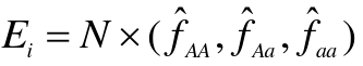
1. Estimate allele frequency (p_hat)
2. Determine the expected genotype frequencies from the estimated allele frequency, assuming null is true
   

   

3. Compute the expeceted genotype counts
   

   

4. Compare observed genotype counted to expected
   

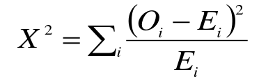
Compare X² to a chi-squared distribution with 1 degree of freedom. This is usually the number of categories minus 1, but we lose an additional degree of freedom since we estimate allelic frequencies from the data (3-1-1).

Conclusion: The observed genotype frequencies are [not] significantly different from the expectations of the HW equilibrium.

When we reject the HWE, we usually don't know why other than the assumptions being violated.

Exact HWE Test

There are (2N)!/n_A!n_B! possible arrangements for the alleles in the sample. Under HWE the probability of observing exactly n_AB heterozygotes in N individuals with nA alleles is: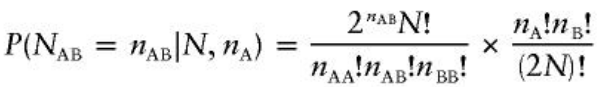

Under many conditions, samples of affected individuals will not be in HWE for alleles associated with disease BUT controls should be close to HWE, as should population-based (unascertained) samples. Note also that genotypes among related individuals may not be in HWE since the individuals are not independent.

If the observed genotypes in unaffected controls (whole random sample) depart from HWE, this may indicate:

• Bad Assay - non-random genotyping error or non-random missing data
• Population structure (non-random mating)

Often if the HWE test p-value is << .01 in controls, the marker is not used in association analyses.

Population Structure

"Random Mating" occurs within a population, but not within overall population.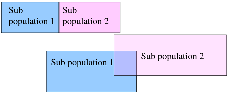

We can observed the combined population to test for structure in sub-populations: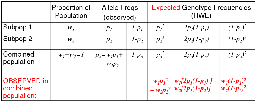

The Heterozygote Deficit = 1 - (observed het freq)/(HWE expected het freq)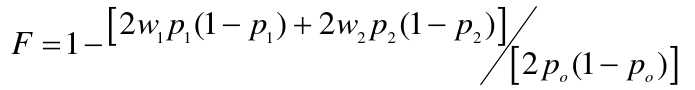
F is the proportional decrease in heterozygotes observed under what would be expected under the HWE.

Linkage Disequilibrium (LD)

Recall a haplotype is a set of markers on the same chromosome that are always inherited together. The haplotype consists of two pieces of information: Genotypes and which alleles are inherited together..

Suppose we have two markers 1, with alleles A and a and freq p_A, p_a, and 2, with alleles B and b and freq p_B, p_b
We have 4 possible haplotypes: AB, Ab, aB, ab
If p_AB is the probability A and B are on the same chromosome, then we can say p_AB = p_{B *} p_b if markers are independent
Let P_t(AB) be the frequency of the haplotype AB after t generations of random mating, and theta is the recombination fraction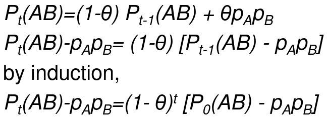

The idea being that we can measure the decay of Linkage Disequilibrium as a function of generations passed: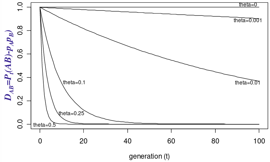

You can also measure this in a pairwise fashion: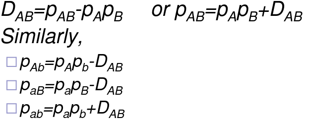

There are problems with the pairwise measure however:

• The sign of D_AB is arbitrary
• Range depends on allele frequencies
• Can't easily compare the different pairs of markers

Min and Max of D_AB:
    If D>0, D ≤ min(p_Ap_b,p_ap_B)
    If D<0, |D| ≤ min(p_Ap_B,p_ap_b)

D is usaully scaled so that its range is (0, 1) or (-1, 1):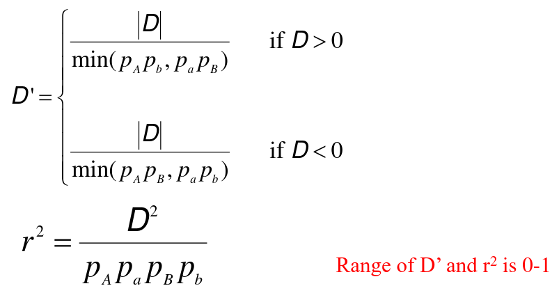

D' = 1 -> No evidence for recombination beteween markers
D' = 1 -> Fewer than 4 haplotypes are observed between two biallelic variants
If allele frequencies are similar D' near 1 -> the markers are good surrogates

D' estimates can be inflated with small sample sizes
D' estimates can be inflated when one allele is rare

Association Testing in Unrelated Individuals

In association testing we are interested in the effect of a specific allele in the population. We ask the question: "Is allele X₁ more common in affected individuals than unaffected individuals?" We do not need family data to answer this, but we can use it if we have it.

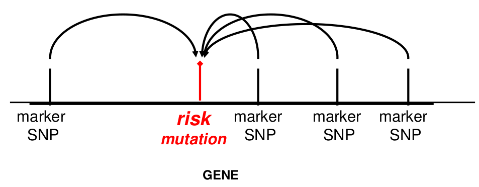
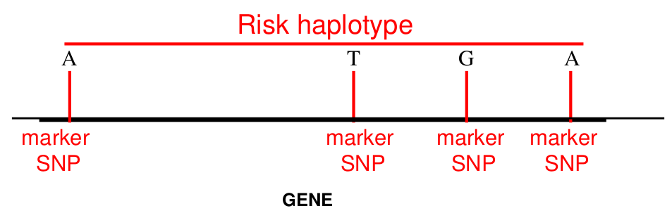
Recall that Linkage Disequilibrium is the tendency for alleles at two loci closely linked on a chromosome to be associated in a population. Linkage is done within a family (referring to alleles inherited together), and LD is done within a population (alleles found at two loci together on a haplotype more often than expected). Two loci are linked when the theta score is less than .5, this does not necessarily mean they are in LD.

After many generations disease causing mutations in LD will change due to recombination.

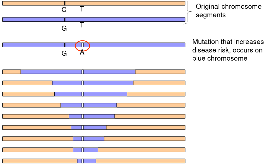
The above graphic represents a mutation on the blue chromosome that over time and recombination through mitosis slowly decreases the LD between the mutation and the surrounding chromosome.

Specific alleles may be functional or in LD with functional mutations.
    Functional = casual -> the mutation that actually causes the increased/decreased risk/phenotype.

Genetic Association Testing

In genetic association analysis, we are trying to identify association between genotype (SNP) and phenotypes. Some alleles may be functional or in LD with functional mutations, meaning it's not the "true cause" of a particular phenotype.

functional/casual - the mutation that actually causes the increased/decreased phenotype

H₀: No association between marker genotypes and phenotype

When the null hypothesis is rejected, we conclude a marker is associated with a phenotype.

The marker may be a functional mutation or in LD with a functional mutation

• Non-synonymous changes, truncation, UTR SNPs may be more likely to be causal ("functional SNPs")
• Synonymous, intronic, IVS SNPs may be less likely to be casual
• Functional studies are usually required to determined whether an associated SNP is functional/casual
• Databases such as ENCODE make it easier to predict if variants have function but its still difficult to be sure for non-exonic variants

Association Testing for Qualitative Traits

• Can be performed within case-control or cohort/population studies
• Case-control commonly used for genetic studies of rare traits
• H₀: there is no association between alleles
• Testing methods:
  • Chi-square (or Fishers exact) test comparing allelic or genotypic frequencies between cases and controls
    • X² = sum((O_i - E_i)^2/E_i)
    • DF = number of genes compared - 1
  • Logistic regression
    • Allows incorporation of covariates
    • Convenient framework for exploration of genetic models
  • For matched case-control studies can perform MH test, conditional logistic regression

Logistic Regression

• Best for regression under a dichotomous outcome (affected/unaffected), when linear regression is not appropriate.
• We want the response (dependent variable) Y to have two possible values, 1 for effected or 0 for non-effected.
• A regression equation can predict a number between 0 and 1 that could be interpreted as the probability of being affected or the log odds of being affected.
• Regression coefficients are the log odds ratios for each of the independent variables.

The linear logistic model has the form: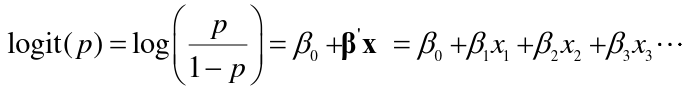

• For a dichotomous predictors the beta parameters in a logistic regression are the log-odds ratios for a disease for those with a risk factor (x = 1) vs those without (x = 0)
• For a continuous or ordinal predictor, the parameters are log-odds ratios for a one unit increase in x.

Coding Genetic Variables

We are interested in evaluating if the genotype at a specific marker is associated with being effected by a phenotype.

Consider a SNP with alleles 1 and 2. We have 3 genotypes, where we het is the heterozygote status and hom is homozygote status of allele 2:

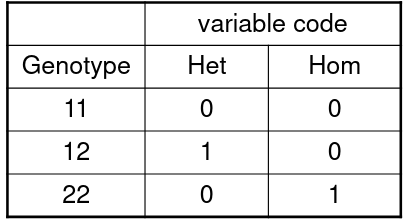
Model: ln(odds for affected | geno) = 𝛽₀ + 𝛽₁Het + 𝛽₂Hom
Our test has 2 degrees of freedom with H₀: 𝛽₁ = 𝛽₂ = 0

So the odds ratio comparing genotype 12 to 11: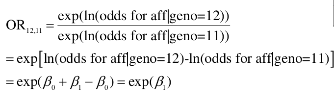Evaluates to be the same as the e to the power of the coefficient of heterozygote variable. We assume is the same as comparing genotype 22 to 12, since we only consider 1 allele at a time.

We can also test if there is a difference between 12 and 22 by creating a dominant and recessive model

Below we look at an additive model where ADD denotes the number of "1" alleles, which we'll assume is more rare than "2" alleles (the reference group):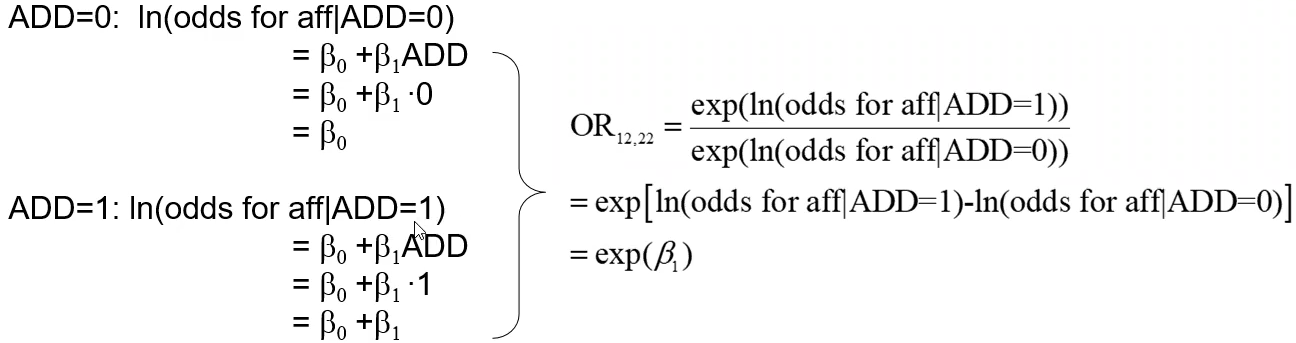

Interpretation

General model:

"The odds of disease for the 12 genotype is OR_12,22 times the odds of the disease for the 22 genotype, and the odds of disease for the 11 genotype is OR_11,22 times the odds of disease for the 22 genotype."

Additive model:

"The odds ratio increases multiplicatively by exp(𝛽₁) for each additional 1 allele"
"The odds of disease increase by a factor of OR_12,22 for each additional 1 allele"
"The odds of disease for the 12 genotype is OR_12,22 times the odds of disease for the 22 genotype and the odds of disease for the 11 genotype is OR_11,22 times the odds of the disease for the 12 genotype."

Determining the Type of Model

Based on Beta Estimates

Compare the beta coefficients from the general model to determine the best genetic model (general, additive, dominant, recessive).

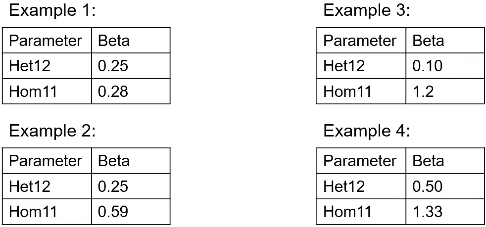1 is dominant because the estimates are nearly the same between heterogygous and homozygous
2 is additive because the het geno is roughly half the hom geno
3 is recessive because there is only an effect if there is a 11 allele
4 is general because it doesn't fit any of the above criteria

Case-Control Tests

Tables vs. Logistic Regression Tests

• Allele-based contingency tables assume HWE (assumes the two alleles are independent and have additive effects).
• Logistic regression with additive model assumes additive effects, but not independence of alleles.
• General model with no covariates in logistic regression will yield very similar results as 3x2 genotype x case status chi-square test.

Cross-Sectional and Cohort Studies

Association Testing for Quantitative Traits

This is typically performed in a random sample from the population. The most common testing method is linear regression; genotypes can be coded exactly as shown for logistic regression. Parameters here are the mean difference in the outcome due to difference in genotype.

H₀: There is no association between alleles (or genotypes) and this trait; 𝛽₁ = 𝛽₂ = 0

From there we pretty much use the same equation as above: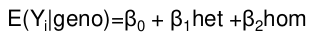

For example, in a table coded identical to the one above, the mean difference in 12 and 11 simplifies to the coefficient of beta for 12 genotype:
𝛽₀ + 𝛽₁ - 𝛽₀ = 𝛽₁

Confounding

Recall that a confounder is a third factor which is related to both exposure and outcome, and which accounts for some or all of the observed relationship between the two.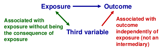

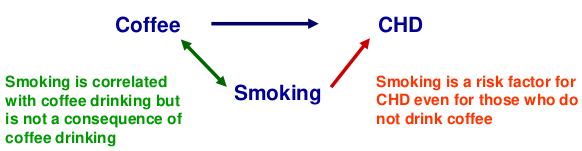
When testing for association between a SNP and phenotype confounders might be population structure, but SNPs are very unlikely to be confounded as behavioral and environmental factors do not alter DNA and vice versa.

Mixing two populations can cause spurious association, or departure from HWE, causing alleles at 2 loci to appear associated even though they may be on different chromosomes.

While it's unlikely to confound in the strict sense, adjustment for behavioral and environmental factors may be helpful if they affect the phenotype independently of the genes of interest. (increased precision of estimate -> increased power)

How to Deal with Structure?

When the sub-populations are known:

• Stratify analyses by sub-populations
• Adjust for sub-population in regression (population dummy variables)

When factors defining sub-populations are unknown or difficult to measure:

• Genetic principal components analysis (requires genome-wide or AIM genotype data)
• Family-based designs: family controls are matched on cases or ancestry

Useful Guidelines

• Race/ethnicity - social categories
  • Influences social factors which influence health
  • Avoid reinforcing the idea that race is that same as genetic ancestry
• Ancestry - genetic origins
  • Influences frequencies of variants in different populations; patterns of LD among variants.
  • Avoid using self-reported race as genetic ancestry

Always explicitly distinguish between variables that derive from non-genetic, reported information vs. genetically inferred information.

Multiple Comparisons and Evaluating Significance

• In 1978 Restricted Fragment Linked Polymorphisms (RFLPSs) were used for linkage analysis.
• In 1987 the first human genetic map was created.
• In 1989 microstellite markers made genome-wide linkage studies possible.
• 1990-2003 the human genome project was sequenced.
• 2002-2006 HapMap project collected sequences in populations to discover variation across the genome.
• 2006 onward, Genome-Wide Association Studies (GWAS)
• 2010 onward, large scale custom arrays
• 2010 onward, sequencing technology becomes affordable
• Even more WGS projects...
  • ADSP 2012
  • TOPMed 2014
  • CCDG 2014

Prior to the GWAS era, genetic association studies were hypothesis driven; Testing markers within/near the gene or region for association. "H0: The trait X is caused/influenced by Gene A." The hypothesis (gene or genes) came from:

• Experiments in other species
• Known associations with a related trait in humans
• Linkage analysis localizing trait to a specific chromosomal region

Chip-based Genome-wide Association Scans

• Hypothesis generating
  • Assumes only that there are genetic effects large enough to find
  • Asks what genes/variants are associated with my trait
• 500k -> 5 million genes/variants across genome
  • Multiple genome-wide chips available
  • Varying strategies for SNP selection
  • Imputation allows testing of ungenotyped SNPs
  • Typically GWAS chips have focused on common SNPs with frequency > 1%

Candidate

• Limits testing to locations of perceived high-prior-probability
• "If you look under the lamppost you can only see what it illuminates"

Genome-Wide

• Extreme multiple testing - requires large sample size, meta-analysis of multiple studies to overcome
• Gives an "unbiased" view of the genome
• Allows unexpected discoveries

Whole Genome or Exome Sequencing

• Identifies known SNPs (that would be on a chip) but also previously undiscovered variants.
• Attempts to assay all, or nearly all, variation in genome or exome
  • Whole exome:
    • ~1% of the genome
    • ~30 million bp
    • Number of variants observed depends on sample size and population
  • Whole genome: 3 billion bp,  > 30 million known variants in 1000G project

Statistical Significance

There many things to test in genetic association studies:

• Multiple phenotypes
• Multiple SNPs
  • Candidate gene or region association
  • Genome-wide association
  • Haplotype Analyses
• Gene-Gene or Gene-environmental Interactions

The multiple tests are often correlated.

Type I error: Null hypothesis of "no association" is rejected, when in fact the marker is NOT associated with that trait.
This implies research will spend a considerable amount of resources focusing on a gene or chromosomal region that is not truly important for your trait.

Type II error: Null hypothesis of "no association" is NOT rejected, when in fact the trait and marker are associated.
This implies the chromosomal region/gene is discarded; a piece of the genetic puzzle remains missing for now.

• The significance level alpha for a single statistical test is the type-I error rate for that test.
• If we perform multiple tests within the same study at level alpha, the type-I error rate specified will apply to each specific test but not to the entire experiment (unless some adjusted is made).
• Probability of a type II error is beta.
• Power = 1 - Beta

For a multiple testing problem with m tests: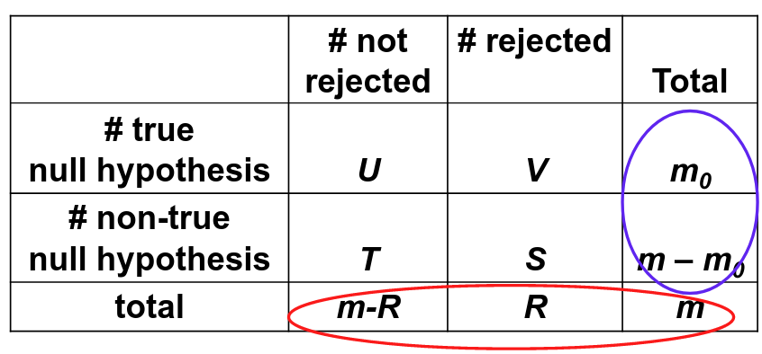

Family-wise error rate (FWER) is the probability of at least one type I error; FWER = P(V > 0)

False discovery rate (FDR) is the expected proportion of type I errors among the rejected hypotheses; FDR = E(V/R)
    Assume V/R = 0 when R = 0

Procedures to Control FWER

The general strategy is to adjust p-value of each test for multiple testing; Then compare the adjusted p-values to alpha, so that FWER can be controlled at alpha.

Equivalently, determine the nominal p-value that is required achieve FWER alpha.

Sidák

Sidák adjusted p-value is based on the binomial distribution:

• Each test is a trial. Under the null hypothesis, the probability of success is p, the significance level that is used
• The probability of at least one success in m trials, each with probability p:
  

  

• For a test with p-value p_i to adjust for m total tests, the adjusted p-value is p_i^* = 1 - (1 - p_i)^m
• This is conservative (over-corrects) when the tests are not independent

Bonferroni

A simplification of Sidák:

Bonferroni adjusted p-value: 

• p_i^* = mp_i
  
• Over-coirrects (conservative) if the tests are correlated

Below are the individual p-values needed to reject for family-wise significance level=.05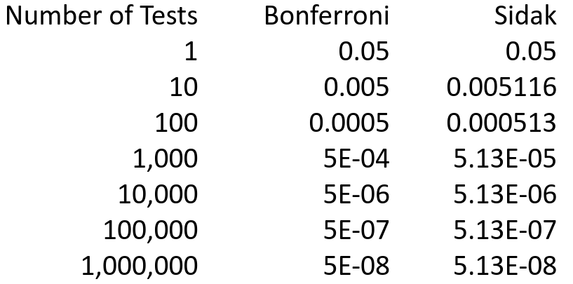

minP

The probability that the minimum p-value from m tests is smaller than the observed p-value when ALL of the tests are NULL.

Equivelent to Sidak adjustment if all tests are independent. But for dependent tests, we don't know the distribution of the p-values under the null hypothesis, so we use permutation to determine the distribution.

Adjusted p-value is the probability that the minimum p-value in a resampled data set is smaller than the observed p-value.

This is less conservative than the above two methods, but the results are equal to Sidak when tests are significant.

Permutation is done under the assumption that the phenotype is independent of the genotypes; and phenotypes are permuted with respect to genotype.
Original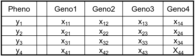

Permuted: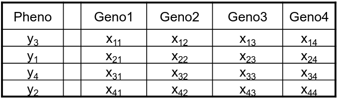

Genotypes from an individual are kept together to preserve LD

Permutation Procedure

• Create 1000+ permuted data sets
  • Identical to the original except phenotype values have been assigned randomly
• Analyze each in exactly the same manner as the original data set
• Determine the minimum p-value from each permuted data set
  • 1000+ minimum p-values
• The minP adjustment: the adjusted p-value is the proportion of minimum p-values that are smaller than the observed p-value.

Permutation is computationally expensive, and in some situations it is not possible at all (related individuals, meta-analysis results).

Alternative

Use the Bonferroni or Sidak correction with the "effective number of independent tests" instead of total number of tests. This reduces the number of tests to account for dependence among test statistics. We must approximate the equivalent number of independent tests.

For a single study you can compute the effective number of independent tests based on the genotype data.

• Use the covariance matrix of all the genotypes that you tested
• Several approaches have been proppsed to estimate the effective number of tests (m_eff)
• Two are best performing:
  • Gao X, Starmer J, Martin ER: A multiple testing correction method for genetic association studies using correlated SNPs
    
  • Li J, Ji L: Adjusting multiple testing in multi-locus analyses using the eigenvalues of a correlation matrix

Once you have an estimate of m_eff use it in the Bonferroni or Sidak correction

Another alternative: Extreme Tail Theory Approximation (not covered here)

FWER Summary

Binferroni, Sidak, minP are all single-step adjustments; i.e. all p-values are adjusted in the same manner regardless of their values. This makes them very easy to understand and compute, however it sacrifices power.

Control FWER is very stringent (< 5% chance of a single false positive)

False Discovery Rate (FDR)

Controlling P(V = 0) is too stringent when m is large and you can expect multiple true positives. For better power,  control E(V/R) instead.

E(V/R) = the expected proportion of Type I errors among rejected null hypothesises.

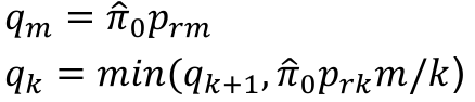
1. Rank p-values p_r1 <= p_r2 <= ... p_rm
2. Adjusted p-values
   
   1. p*_rm = p_rm
   2. p*_rk = min(p*_rk+1, p_rkm/k)

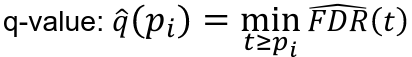
FDR: Q-Value

For an individual hypothesis test, the minimum FDR at which the test may be called significant is the q-value. It indicates the expected proportion of false-positive discoveries among associations with equivalent statistical evidence.

FDR for a specific p-value threshold t: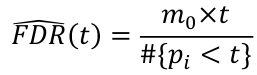
where m₀ = number of true null hypothesis

We can estimate m₀ by m*pi_hat_0; where pi_hat_0 is an estiamte of the proportion of true null hypothesises (could be ~1)

1. Rank p-values: p_r1 <= p_r2 <= ... p_rm
2. Estimate the proportion of true null hypothesises pi_hat_0
   1. Using pi_hat_0 = 1 leads to conservative q-values estimates equal to the FDR adjusted p-values
   2. See suggested approach in Story and Tibshirani (2003)
3. Compute q-values:
   

   

4. Reject null hypothesis f q-value <= alpha

Which to use?

• Bonferroni and Sidak
  • Almost no assumptions
  • No permutations required
  • Use when number of tests is small or power is not an issue, or if a quick computation is needed
  • When number of tests is moderate and correlation structure of tests or SNP uses:
    • Extreme tail theory
    • Benferroni adjustment with number of effective independent SNPs
• Permutation approach
  • Does not assume independence of SNPs
  • Use when computationally feasible
• FDR or q-value
  • Controlling E(V/R) instead of P(V > 0)
  • Useful for exploratory analyses with a large number of markers/models/subgroups to test
    • FDR and q-value thresholds are often set higher than traditional (.05) level
  • First proposed for analyzing micro-array data
    • Works best when the proportion of null hypotheseses expected to be rejected because they are false is not too small.

Guidelines for Adjusting for Multiple Comparisons

• Genome-Wide Association Study (GWAS)
  • Must adjust for all tests performed to claim experiment wide significance
  • Common strategies:
    • Staged Design:
      • Stage 1: GWAS on subset of available subjects
      • Stage 2: Independent sample/subset, test only the small subset of SNPs that were significant at some level in Stage 1
    • Meta-analysis of multiple studies
      • Each study performs GWAS
      • Results from all studies are combined
    • Combination of these two approaches
• Staged GWAS
  • Two alternatives for multiple testing correction
    • Replication: Analyze Stage 2 separately, adjust stage 2 for number of tests in stage 2
    • Joint analysis: Analyze stage 1 and 2 jointly for SNPs genotyped in stage 2, adjust joint analysis for all SNPs tested in stage 1
  • Usually joint analysis strategy more powerful
    • Joint analysis is more efficient than replication based analysis at two stage genome-wide association studies.
• GWAS meta-analysis
  • For each SNP, combine results from all studies
  • Similar in power to a study with sample size = sum of all sample sizes
  • Significance levels appropriate for single GWAS are appropriate for meta-analysis GWAS
• Candidate gene studies
  • Often we will test SNPs that have already been associated in other independent studies
  • Whether the candidate genes were chosen based on prior association, linkage or relevance of any kind
    • must adjusted for all tests performed in your study to claim experiment-wise significance for any one SNP

Overall: we are unlikely to have sufficient power to achieve experiment-wide or genome-wide significance with a single study, large number of SNPs

Best choice is meta-analysis and/or replication using independent studies

When combining studies is not an option, report the most promising results based on p-value and other factors

Make available results from all SNP association analyses so that other investigators can attempt to confirm or repliucate your findings.

Choose a threshold BEFORE looking at the data.

Genomic Control

Genomic control was preposed to measure and adjust for modest population structure within a sample in the context of GWAS

• Most SNPs that are tested in a GWAS (which is most) are not associated with the trait
• Association tests from random sites in the genome shouhld be distributed as if a set of unassocaited (null) tests
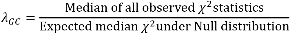
• The genomic control inflation factor 𝜆_GC or just 𝜆, is defined as:
  
• Typically estimated using the entire set of GWAS variants
• 𝜆 is a measure of the inflation of test statistics in your GWAS
  
• If your study has population structure then the unassociated test statistics will not follow the null distribution.
  • On average, each statistic will be a bit "too big"
  • The median of the test statistics will be larger than the median test statistic from the null distribution, so 𝜆 > 1
• 𝜆 can also be used to deflate test statistics so that the observed median matches the expected distribution
  
  • Compute 𝜆
  • Divide all test statistics by 𝜆 before computing p-value
• GC correction assumes that all the GWAS test statistics are inflated an equal amount

PLINK outputs Z statistics in the STAT column, but 𝜆 is calculated from chi-square test statistics. Z² is a chi-square statistic with 1 degree of freedom. We can transform the p-value from plink into chi using the qchisq() function in R.

 

Association Testing in Related Individuals

Family data is correlated that could lead to inflation in test statistics if not accounted for. Many genetic studies contain related individuals. Family-based studies were developed to avoid bias due to population structure; Biological family members are genetically matched.

Most behavioral and environmental factors do not alter DNA, so SNP associations are unlikely to be confounded EXCEPT confounding by ancestry.

Population Stratification Bias

• For case control studies, population structure means bad matching; cases and controls come from different genetic populations.
• For cohort/cross-sectional studies with quantitative phenotypes, if the phenotype and genotype distributions both differ by population then population stratification bias can occur.
• If a population consists of a mixture of subpopulations and it is not accounted for in the analysis, false evidence for association may result.
• Spurious association only occurs when there is a difference in BOTH genotype and phenotype distribution with subpopulations.

Designs for Family-Based Studies

• Early-onset phenotypes:
  • Case-parent trios (where child is effected) - Transmission disequilibrium test (TDT)
• Late-onset phenotypes:
  • Discordant siblings - sub-TDT/conditional logistic regression
• General designs
  • Nuclear or extended families - Family-based association test (FBAT)

We'll mostly focus on case-parent trios and TDT tests.

Case-Parent Trios

In this design we collect samples of trios; Two parents and one affected child (affection status of parents are not considered). The idea is under Mendels laws, heterozygous parents transmit each allele with equal probability (1/2) regardless of population structure. If there is preferential transmission of a specific allele from parents to affected offspring it indicates that allele is associated with the disease.

Transmission Disequilibrium Test (TDT)

Tests whether a particular marker allele is transmitted to affected offspring more frequently than expected. Non-transmitted alleles act as matched controls.

H₀: No association or no linkage
H_a: Variant is associated with disease/trait (and is not due to population structure)

Notation:

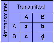
• a = number of AA parents
• b + c = number of AB parents
  • b = Number of AB parents transmitting B to affected child
  • c = Number of AB parents transmitting A to affected child
• d = number of BB parents

Under the null we would expect: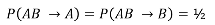

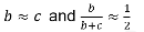
The test statistic follows a McNemar test:

We observe this is only a function of the heterozyzgous parents, homozygous parents provide no information.

Discordant Siblings

• TDT unit of analysis is affected child + parents.
• Discordant siblings - unit of analysis is sibships with at least one affected and one unaffected sibling
• Analysis possibilities:
  • Cochram-Maentel-Haenszel test
  • Conditional Logistic Regression
• Like TDT these tests are conditioning on the genotypes in the family
  • TDT: conditioning on the parent's alleles
  • Sibs: conditioning on the observed genotypes in the sibship

General Family Structures

• Family Based Association Test (FBAT) and other similar tests (requires specialized software)
• Determine the expected genotypes of the affected individuals conditional on the family structure
• Use this to create a score test comparing observed and expected genotypes
• Same idea as parent-offspring trios or case-control sibships: conditioning on the observed genotypes

Unconditional Tests

• TDT, sTDT, FBAT and other family based association tests are conditional tests
• These tests are immune to population structure bias but often ignore information that can be used to assess association when population structure is not a concern
  • Homozygous parents
  • Sibships where the case and control have the same genotype
• Modern analyses can account for population structure using ancestry information available with genome-wide data
• Unconditional analyses account for the family correlation and make use of all the observed data
• These analyses tend to be more powerful than the conditional family-based tests

Review: For unrelated (independent) subjects we can use standard linear or logistic regression. Including related individuals in the analysis violates the assumption of independence, causing inflation in the test statistics.

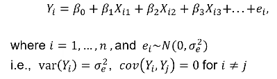
Where X_i1 is the genotype of the i^th person and beta1 is the fixed affect of the SNP. X_i2 and X_i3 are covariates.

For related data there are specific methods we can use:

• For quantitative traits use Linear mixed effects models are frequently used for corrected observations for an individual or related individuals.
• Pedigree-specific methods use a variance component that is dependent on the kinship matrix for individuals.

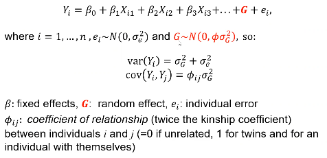
We can see the mixed effects model adds a G variable to account for genetic variance component.

For association analysis of quantitative traits, if X₁ is the SNP then the test H₀: Beta1 = 0 is a test of association just as for the linear model for unrelated subjects. The regression estimate beta is exactly the same as in simple linear regression.

In either case G is not tested for significance. If we want to test for heritability we estimate variance of G.

Common software: GCTA, SOLAR, R GMMAT package, Genesis R/Bioconductor package.

Dichotomous Traits

• Logistic mixed effects can be used to account for relationships
  • Fit using penalized quasi-likelihood method
  • Requires iterative matrix inversion - can be very slow
• Alternative: Logistic model with Generalized Estimating Equations (GEE)
  • Accounts for correlated observations in a general way
  • Produces a "robust" variance estimate to account for correlation
  • Tends to result in inflated Type-I error
    • Low frequency SNPs primary probelm
    • Extent of inflation varies

In this course we focus on quantitative traits to keep things simple.

Haplotypes and Imputation

When multiple markers/SNPs are genotyped in a gene or gene region, the SNPs may be in linkage disequilibrium (LD). Each individual test of association with a marker is correlated with all tests for other markers in LD with that marker.

So, instead of testing the individual markers for association, we may want to test haplotypes of markers for association.

Review: A haplotype is a combination of alleles at multiple loci that are transmitted together on the same chromosome. It should provide the alleles present on the locus and which alleles are on the same chromosome. For example, if we have 2 SNPs with alleles (A, a) and (B, b) then we have 2x2= 4 possible haplotypes: AB, Ab, aB, ab.

For linked SNPs within a gene or small chromosomal region there are typically far fewer haplotypes observed than are theoretically possible (as a consquence of LD).

Reasons to Care About Haplotypes

1. We haven't typed the casual variant. The haplotype that the variant lies on is a better surrogate for the variant than any one SNP in the haplotype.
   

   

2. The "causal" genetic variant is actually the haplotype, not any one variant -- The haplotype confers risk rather than an individual SNP allele.
   

   

3. They allow us to impute additional ungenotyped variants

Often we don't have family data to help us. Haplotype phase is ambiguous only if there are 2 or more heterozygous genotypes. For example, Aa Bb genotype has two possible phases: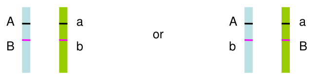

All multi-locus genotypes that consist of 2 or more heterozygotes have ambiguous phase.

When family data is not available to determine haplotypes, multi-locus haplotype probabilities and frequencies can be estimated.

Haplotype Inference

The goal is to get the probability of a haplotype given the individual's genotype. There are two classes of algorithms: EM or MCMC

• EM requires HWE assumption; MCMC does not
• EM algorithm is memory demanding to infer haplotypes for a large number of SNPs; MCMC method requires much less memory but more time

There are many options for software for phasing with and without family data.

The basic idea is to determine haplotype frequencies for sets of SNPs in close proximity on a chromosome, and compare frequencies in cases and controls or by quantitative phenotype.

Which SNPs should we use to test with Haplotypes?

• Options include:
  • All SNPs on a chromosome
  • All SNPs on a "haplotype block" (chromosome segment where all variants are in high LD)
  • Sliding windows of 2-5 SNPs across region of interest
• Unless there is high LD, there will be more haplotypes than SNPs -> create haplotypes from SNPs that are in LD

Regression with Haplotypes/Likelihood-Based Tests

Take the following example with 3 SNPs and 4 observed Haplotypes, where each person i has 2 haplotypes: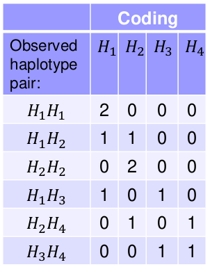

We can use variables to count the number of each haplotype type per person. This coding works for any type of multi-allelic marker, not just haplotypes.

We can use a linear regression model with the haplotype counts as predictors:

Note we do not include H₁ in the model. Since H1 + H2 + H3 + H4 = 2, we already know H1 once we know the remaining haplotypes. Think of H1 as a reference haplotype.

Each individual will have a 0, 1, or 2 for each of the 3 indicator variables for the haplotypes.

For 4 haplotypes, the general (Omnibus) test for association would be:
H₀: Beta1 = Beta2 = Beta3 = 0; df = 3
If we reject the null, the do tests on individual haplotypes

Global (omnibus) tests of haplotype association provide some protection from  the multiple testing problem, as it tests whether the haplotype distribution is associated with phenotype.

In reality we rarely know haplotypes with certainty. Instead, for each individual haplotype estimation produces the probability of each possible haplotype pair. Can use the same model, but replace the observed haplotype counts with the expected counts (determined by probabilities).

SNP Imputation

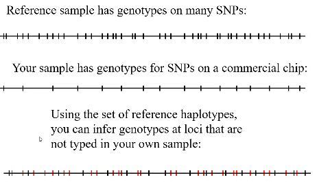
The most recent application of haplotypes is imputation. The idea is we use a reference population that has denser genotyping of whole genome sequencing on your subset of SNPs plus many additional SNPs to impute the SNPs not typed on your chip.

A reference population is a set of individuals who have been genotyped or sequenced in a comprehensive manner. Typically these are for the whole genome sequenced (all the SNPs are included in the sample, plus many additional).

The HapMap project was the first available reference population. HRC created a large reference panel of human haplotypes by combining together sequencing data from multiple cohorts (current release consists of 64,976 haplotypes at ~39 million SNPs). TOPmed has a set of haplotypes from 97,256 genome sequenced individuals, more diverse than HRC.

The two commonly used methods for imputation are IMPUTE and Minimac, and some organizations have "imputation servers" so you can impute your GWAS data to large sequenced data sets without needing powerful on-site computers.

"Dosage"

Genotype imputation does not assign a genotype to each individual, instead for each individual it assigns a probability for each of the possible genotypes at each genetic variant.

Analysis is then performed on the "dosage" - the expected genotype. The most common model is additive, but one could also use a dominant or recessive dosage.

"Best Guess Genotype"

Another method is "best guess" genotype. This is the genotype with highest probability. It ignores uncertainty in genotype assignment. We usually impose a posterior probability threshold; If p < Q, genotype is set to missing (typically set to .8, .9 or .95)

Imputation Accuracy

The overall quality of imputed data depends on how well matched the reference samples are to the samples you are trying to impute.

The concordance of imputed genotypes with true (unknown) genotypes also depends on how much information about the ungenotyped SNPs (how strong is the LD between ungenotyped and genotyped SNPs?)

For high information the concordance reaches nearly 100%, for low information regions it can be much lower.

Imputation R² is an estimate of the squared correlation between imputed and true genotypes. It can be estimated by the obs/exp variance ratio: ratio of empirical genotype dose variance to expected (binomial) genotype variant.

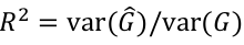
Due to excess homozygosity in a well imputed variant, R² will occasionally be more than 1.

This imputation quality measure is also a measure of the correlation between the imputed genotypes and true gentoypes. 

Typically:

• R² >= .8  is good imputation
• R² < .3 is bad imputation
• .3 >= R² < .8  is moderate quality imputation can be used in analysis
  

Good imputation:

• Has a imputed genotype dosage close to the individuals true (unknown) genotype
• Allele frequency estimated from the imputed genotypes is close to the true frequency
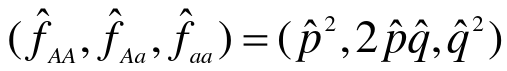
• Under HWE, genotypes should have frequency q², 2pq, p² and genotype variance 2pq (binomial distribution)
• The best possible imputation will have a sample variance of G_hat which is the same as the binomial variance, and R² = 1

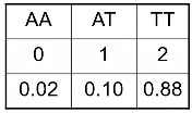
The worst possible imputation is when we have no information about the genotypes other than the allele frequency (which can be estimated from the reference haplotypes). In this case, the imputation would assign everyone the genotype probabilities q², 2pq, p².  Thus everyone would have the same genotype dosage: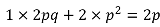

Variance would be 0 because there is no LD between SNPs, and thus correlation would be 0.

Why Impute Genotypes?

• Fill in missing genotype data
• Can test ungenotyped SNPs (with some error) for association
• Analysis of individual SNPs are easier to interpret than haplotypes
• Simplifies combining results from genome-wide association studies using different genotyping platforms

We can also combine studies to increase sample size, and thus the power. The problem is when studies use different reference SNPs, which is why the common SNPs across platforms is small. There are 2 ways to combine studies:

• Combined (joint or pooled)
  • Combine individual data from multiple cohorts
  • Often not feasible because of patient confidentiality
• Meta analysis
  • Combining evidence for assocation across studies
  • Can combine test statistics, p-value or effect size estimates (i.e. regression parameters)

 

 

Power and Sample Size Calculations for Association Studies

Review of errors and difference in means/proportions: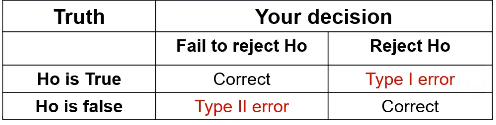

Type II error is represented by beta and type I error as alpha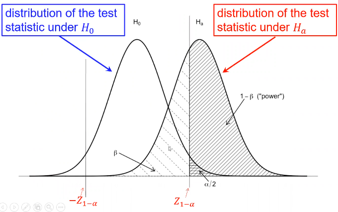

Where Z_{1 - (alpha /2)}is the Z-value that creates the target value of alpha in the tail of the distribution. Power decreases as alpha increases.

Power also has a direct relationship with sample size. Sometimes we choose sample sized based on the desired power for a specific alternative hypothesis of interest, and other times we used a fixed sample size and significance level.

A Z-test of differences in proportions with 2 groups with different sample sizes: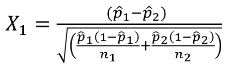

C is the mean of the distribution under the alternative hypothesis: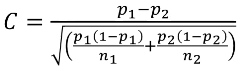

And the power can be calculated by taking the cdf of C minus the one sided Z-value

Likewise, we can use a similar z-test for differences in the mean of a quantitative trait: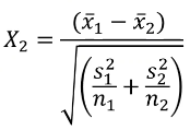

And the power can be calculated the same way as proportions.

Applying Power to Genetic Associations

• Difference in proportions: we can compute the power for a test that  compares the allele or genotype frequency between cases and controls
• Difference in means: we can compare the mean trait values between individuals with different genotypes at a marker (and we can extend this to an F-test for a linear regression)

Dichotomous Traits

1. Determine the expected genotype frequencies in cases and controls under the alternative hypothesis of interest
2. Estimate power for given sample size or estimate minimum sample size required for given power and significance level under the planner analysis model

Genetic Model

• We usually use 4 parameters to specify the disease model for a dichotomous trait:
  • Genotype relative risks y₁ and y₂
  • Population prevalence of disease K
  • Risk allele frequency q (the allele that increases risk of disease)
• To compute power, we need the genotype frequencies for cases and controls under the alternative hypothesis
  • P(personal carries i risk alleles | affected)
  • P(Person carries i risk alleles | unaffected)
  • for i = 0,1, and 2

Genotype Relative Risk

Another way to parameterize penetrance, the probability that someone is affected given their genotype.

Penetrance f_i = P(affected | i risk alleles) for i = 0,1, or 2 risk alleles at a locus

• f = (f₀, f₁, f₂) is the penetrance for the genetic variant.
• f₀ = f₁ = f₂  if there is no difference in probability of being affected by genotype -> the genotypes at this variant are not associated with case status
• If at least one f_i != f_j -> the genotype at this variant are associated with case status
• The genotype relative risks (GRR) are ratios of the penetrance values
• y_i is the ratio of probabilities of being a case for someone with i risk alleles compared to someone with 0 risk alleles
  • y₁ = f₁/f₀
  • y₂ = f₂/f₀
• y₁ = y₂ = 1 -> f₀ = f₁ = f₂ -> No difference in probability of being a case between genotypes with 1 or 2 risk allele(s) and 0 risk alleles -> no association between case status and genotype
  

So if we know the relative risks (y₁ and y₂), the population prevalence K, and the risk allele frequency q, we can determine the penetrances (f_0, f₁, f₂):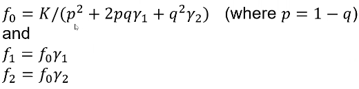

This is derived from the law of total probabilities which I will not show here.

Models for Dichotomous Traits

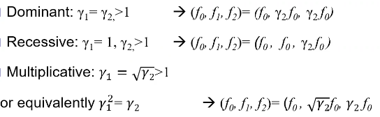
Note: multiplicative GRR ~= multiplicative OR
additive log(OR) -> multiplicative OR
Thus, multiplicative GRR model is most similar to the additive log(OR) model that we use in logistic regression

H₀: Genotype or allele frequencies are the same in cases and controls
Ha: genotype frequencies are not equal in cases and controls. They follow a [dominant, recessive, additive] model

To compute power we need the genotype frequencies for the cases and controls under the alternative hypothesis:
P(i risk alleles | person is a case)
P(i risk alleles | person is a control)
For i = 0,1,2

The expected genotype frequencies for cases and control from f using Bayes Rule: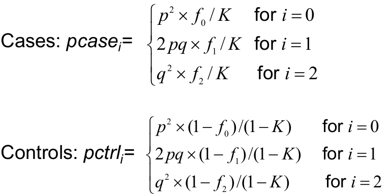

To compute power we not only have to specify the alternative hypothesis model, but also choose the model you will use to do the analysis. The analysis model is the model you choose for the analysis for which you compute power.

Under a dominant model the genotype relative risk should be y₁ = y₂ = 2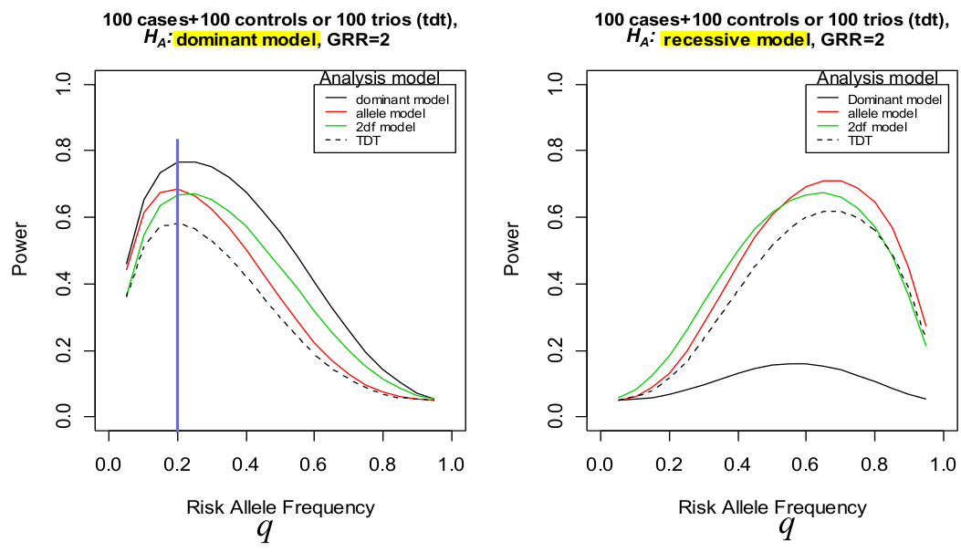

Notice how when we analyze the recessive model as a dominant one (right), the power decreases significantly.

Power - General 2DF Test

We can also compute power for the 2df genotype-based chi-squared test. The underlying formulas will not be explained here as there is software to compute this called the Genetic Power Calculator; You specify GRRs, prevalence risk allele frequency and it produces the genotype frequencies in cases and controls and the power under dominant, recessive, additive and 2DF tests.

Summary - Power for Dichotomous Traits

1. Determine the expected genotype frequencies in cases and controls under the alternative hypothesis
   • Need to specify genetic model/effect size
2. Estimate power for given sample size or estimate minimum sample size required for given power using the specific analysis model and significance level
3. Can also find the minimum effect size that yields specific (usually 80%) power for a given sample size and allele frequency

Quantitative Traits

We usually parameterize power for quantitative traits in terms of locus-specific heritability (h²), the proportion of variance explained by the genetic variant (R²). It is independent of underlying model and allele frequency.

For a linear regression F test, the power is determined by the non-centrality parameter 𝜆, the proportion of variance in the trait explained by the genotype (h²) * sample size

𝜆 = h² * N

To determine the (central) F distribution:
    In R: qf(1-alpha, df1, df2)

Code to determine power using non-central F-distribution and non-centrality parameter "ncp":
    In R: pf(crit.val, df1, df2, ncp, lower.tail = F)

So for any proportion of variance explained by h² and N we can compute power. However, a single h² value corresponds to many alternative hypothesis models.

For dichotomous traits we can simply compute power for difference in proportions, but specifying an underlying genetic model (GRRs, prevalence, allele frequency) is more meaningful. Similarly, power for a quantitative trait is usually more meaningful if we understand how the heritability relates to the genotypic means for a trait -- the genetic model. To find this we need allele frequency for that allele that increases phenotype and the degree of dominance d (additive, dominant or recessive).

Genotypic Means

a is effect size

Recall the variance components in a single gene model: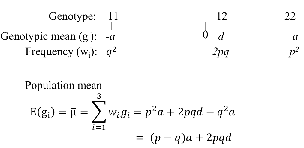

Locus-specific heritability h², degree of dominance d, and allele frequency p: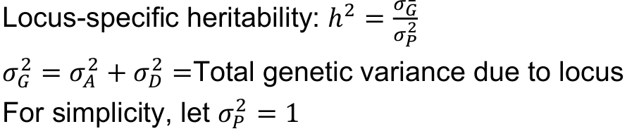

We can re-scale so that the total trait σ²_P = 1, by dividing the trait values by SD: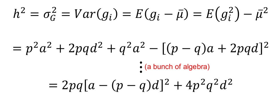

Next we can set R = (-1, 0, 1) for recessive, additive and dominant models respectively, then d = Ra. We substitute Ra for d in the above and solve for a: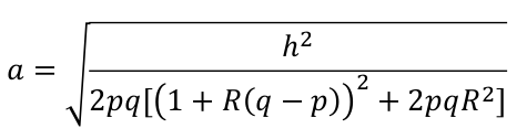

When R = 0: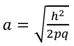

Recap on Effects on Power

• Dichotomous Traits (difference in proportions) are effected by:
  • Effect size: Model (dom/rec/add...)
  • GRRs
  • Risk allele frequency
  • Prevalence of disease/distribution of phenotype
• Quantitatice Trait
  • Effect size: Proportion of variance explained by the genetic variant is affected by:
    • Model (dom/rec/add...)
    • Allele frequency

Use a significance level you will use when performing association tests, or the entire family-wise error for the entire experiment.

For the model, if there is no prior hypothesis, try to find examples from the literature of reasonable effect sizes for your alternative hypothesis. Usually under an additive or multiplicative model. Beware that differences in study design can lead to different expected effect sizes.

Winner's curse is when significant regression estimates from small underpowered samples are biased -- tend to over-estimate the true effect.

Sequencing Data and Analysis of Rare Variants

Genotyping arrays can be obtained at pre-selected sites for each sample. Ex. Genotyping sites known to be polymorphic based on prior sequencing.

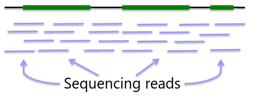
Sequencing is obtaining "every" base in the exome or genome for each sample. Most of the sequence is identical across samples. This is used to find locations that are polymorphic, or differ across samples.

Whole Genome Sequencing

Genome: ~3GB per individual

Advantage - whole genome coverage
Disadvantage - cost ~$1000 for 30x, limited interpretability

Whole "Exome" Sequencing

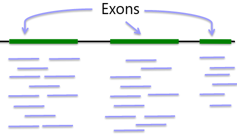
Exome: ~33MB per individual

Advantage: Covers protein coding regions, interpretable variation, cost ~$500
Disadvantage: Missing 99% genome coverage

VCF Format

Variant Calling File (VCF) is a standard format for storing sequencing data. It includes genotypes for all sites where at least one individual had alleles different from references alleles for all individuals in the study.

Every VCF file has three parts in the following order:

• Meta-information lines or Header (begins with ##)
• Last Meta-information line: Record Header (line beginning with #CHROM)
• Data lines (Body) contain marker and genotype data (one variant per line)
  • A data line is called a VCF record
  • Each VCF record has the same number of tab-seperated fields as the record header line
  • The symbol "." is used to denote missing data

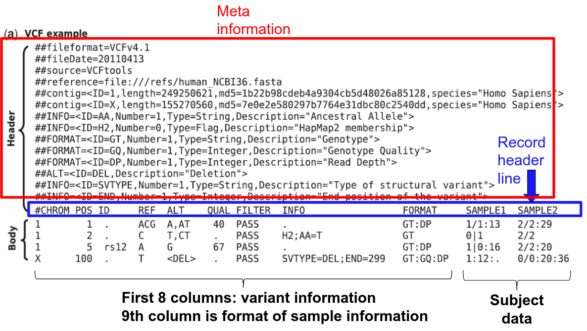
The first nine columns of the data record give information about the variants:
1. CHROM – the chromosome number/id
2. POS – the genome coordinate of the first base in the variant.
Within a chromosome, VCF records are sorted in order of increasing position.
3. ID – a semicolon-separated list of marker identifiers (often rsid)
4. REF – the reference allele expressed as a sequence of one or more A/C/G/T nucleotides (e.g. "A" or "AAC")
5. ALT – the alternate allele expressed as a sequence of one or more A/C/G/T nucleotides (e.g. "A" or "AAC"). If there is more than one alternate allele, the field is a comma-separated list of all alternate alleles.
6. QUAL - The Phred-scaled probability that a REF/ALT polymorphism exists at this site given sequencing data. A value of 10 indicates a 1 in 10^1 chance of error, 50 indicates 10^5 chance of error, etc.

7. FILTER - Either "PASS" or a semicolon-separated list of failed quality control filters
8. INFO - Values in INFO are defined in the header. Contains additional information about the variant represented as tag-value pairs, where the tag and value are separated by an equals sign, and pairs are separated by colons. Usually it is information summarized from the samples, but can also include information from other sources such as population frequencies from a database.
9. FORMAT - Explanation of information in FORMAT are defined in the header. As for INFO, a colon-separated list. Describes the format of the data reported for each sample in the file.

There are many tools that can be used with VCF and BCF (binary version of VCF), such as bcftools and plink.

"Missing Heritability"

GWA studies are great for identifying SNP associations, but usually loci identified have small effects on traits. Much of the phenotypic variation or risk due to genetics ("heritability") is unexplained.

Unexplained variance/risk may be due to:

• Many additional variants with very small effects
• Non-SNP variants such as structural variants not typed by current GWAS chips.
• Epigenetic factors: methylation
• Over-estimation of heritability due to:
  • Genetic interaction
  • Dominance effects
  • Shared environment
• Rare variants that we have have not yet been tested

Rare Variants

There are a lot of different rare variants, they are very common! Rare variants are more likely to be functional/deleterious. The best way to find rare variants is to sequence.

Recent expansion of the human population supports the theory of causal rare variants (there's 8 billion people today). Multiple causal rare variants have been found within genes. Animal studies suggest larger effects of rarer variants.

MAF (Minor Allele Frequency) cutoff can be used to define a "rare" variant (this level makes a difference in analysis).

Association Analysis with Rare Variants

The problem with single variant tests such as regression methods is that there are too few observations to provide a stable test.

We can combine rare variants by grouping them by gene region or functional information (exomes, non-synonymous or nonsense, predicted function), which can improve power.

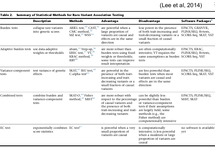
Burden Tests

• Instead of testing rare variants individually, group variants likely to have similar function
• Score presence or absence of rare variants per individual -- use rare variant score to predict trait values
• Makes the assumption that the effect of all rare variants is in the same direction
• If all variants grouped in a test are causal, leads to a large increase in power
• Success (power) depends on:
  • Number of associated variants contributing to signal
  • Number of neutral (null) variants
  • direct of effects

CAST

• Compare the frequency of cases and controls with at least one mutation within a gene or region
• Can be thought of as an indicator approach
  • Xi = 1 when subject i has at least one rare variant in the region/gene
  • Xi = 0 when a subject i has no rare variants
• CAST score can be tested against any type of outcome in regression framework
• Assumes same effect whether a single or multiple rare variants occur in a region in an individual

Unweighted Sum / CMC

• An extension of CAST
• An unweighted sum of the rare variants in a gene or region
  • Commonly used to collapse rare variants into a score of minor alleles
• Regression (linear or logistic) used to test association with the rare variant score (sum)
• All variants included in the sum are assumed to have the same magnitude and direction of effect

RVT1

• An extension of CAST/CMC
• Instead of the sum, uses the proportion of sites at which an individual carries a rare variant as the predictor
• Accounts for missing data:
  • n_i - Number of rare variants for which subject i has been genotyped
  • r_i - Number out of the n_i sites where individual i carries at least one rare allele
  • Score is r_i / n_i

Weighted Sum of the Variants

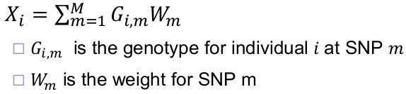
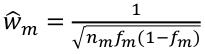
Risk Allele Frequency:

For case-control outcomes: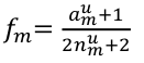

a_m: total number of minor (or risk) alleles for the SNP m
n_m: total number of subjects for SNP m
a^u_m: number of minor (or risk) alleles in the unaffected subjects for SNP m
n^u_m: total number of unaffected subjects for SNP m
G_i,m: is the number of risk variants for SNP m in individual i

Madsen and Browning proposed using a weight based on the inverse of the MAF in the unaffected sample. Lower MAF SNPs have a larger weight. Makes the assumption that the rarer variants have a large phenotypic effect.

• Weights can be developed using any criterion; Allele frequency, function, previous evidence. There is no "best" way
• Use weight in a regression to include covariate and use for quantitative outcomes
• Allows variants to be treated differently based on beliefs about likelihood of functionality
• Still assumes all variants have effect in same direction

Variable Threshold (VT) Model

• Addresses arbitrary MAF cutoff of other burden tests
• Calculates test statistics across many MAF cutoffs
• Chooses maximum test statistic over all MAF cutoffs
• Controls for over fitting using permutation
  • Computationally expensive
• Regression framework -- quantitative or qualitative outcome, covariates
• All variants in MAF bin have the same direction of effect: Weights:
  • 0 for variants that are excluded based on MAF
  • 1 for variants included

Variance Component Tests (SKAT)

Sequence Kernel Association Test

• Test of the joint effects of multiple variants in a region on a phenotype
• Regression framework: allows for inclusion of covariates
• Does not require permutation
• Does not get an estimate of effect size (beta)

We want to test H0: Beta_1 = Beta_2 = ... = Beta_m  Or   t = 0
Assume: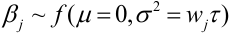

t is a variance component and w_j is a pre-specified weight for variant j, usually chosen to be a function of the MAF.

Under the null hypothesis Q is a mixture of chi-squared distributions.

Variance component score test statistic:

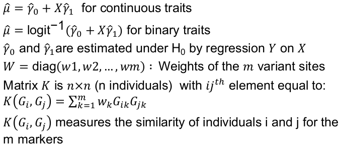
For the weights the original paper recommends this weight for variant j:
wj = Beta(MAFj, alpha1, alpha2), with alpha1 = 1 and alpha2 = 25 or Madsen-Browning uses alpha1 = .5 and alpha2 = .5

SKAT-O

The goal is to combine the best features of SKAT and burden tests into one test with optimal power. Burden tests have good power when all variants have similar effect size & direction. SKAT has better power when many variants are null and/or effects in opposite directions.

• Unified test statistic is a weighted sum of the burden test statistic Q_B and the SKAT statistic
  

  

• The weight sigma can be interpreted as the correlation of regression coefficients of the variants
  • If close to 1: collapse all variants and use burden test
  • If close to 0: all different, SKAT is most powerful
• Asymptotic distribution is mixture of chi-square 1df (for Q_B) and mixture of chi-sqaures (for Q_S)
• P-value can be computed analytically with numerical integration

Significance Thresholds for Rare Variant Tests

Depends on:

• Type of sequence study
  • Targeted
  • Exome
  • Whole genome
• Type/numbers of tests performed
  • One test per gene
  • Multiple tests per gene -- whether different or same tests were run on SNP sets
  • Are the tests independent
• Testing a region already known to have a signal
  • Using independent samples
  • Using the same samples that identified the region

Bonferroni for the number of tests performed can also be applied. Though it is likely to be conservative, even if tests are independent -- some tested genes/regions do not have sufficient variation. Unless the study is very large, p-values likely to be less significant than expected under H0: no association.

Conditional Analysis

For regression-based tests, a conditional analysis amounts to including the associated common variant AND the rare variant score in the same model.

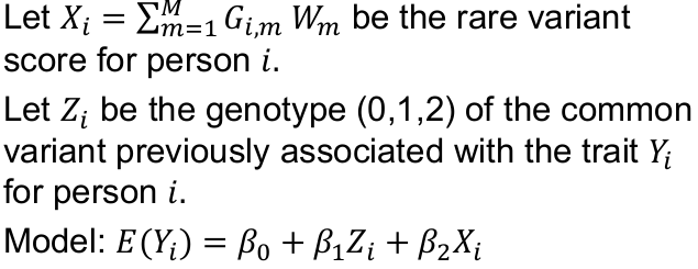
To test whether the rare variant score is associated with the trait conditional on the common variant:
H0: Beta_2 = 0

If the test is significant then the association between Yi and common variant Zi does not fully explain the association observed between Yi and rare variant score Xi, i.e. the rare variant is not just a proxy for the common variant or vice-versea.

 

Interactions in Genetic Assocation Analysis

Statistical interaction occurs between two factors if their combined effect is different than what would be expected based on their individual separate effects. In genetics, differences in risk or mean phenotype between genotypes vary according to the exposure (interacting) variable.

Simple example: Phenylketonuria (PKU) is a genetic defect that causes severe intellectual disability only in the presence of dietary phenylalalnine. Every baby is tested for this trait to see if they need a special diet.

Modeling Statistical Interaction

We need a model to form an expectation for the joint effect, which we can use to define the interaction. The definition of interaction relies on some specification of non-interactive effects.

Let G_i be the genotype for person i, and E_i be an environmental factor for a person i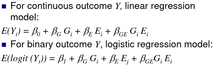

H₀: β_GE = 0; No interaction, the measure of association β_G between the distribution of the phenotype Y and the genotype G does not depend on E.

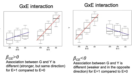
• Model interaction is always written as a departure from additive effects
• For both logistic and linear regression, this translates to departure from additivity of effects
• For logistic regression
  • Interaction == departure from additivity of log(ORs)
  • This is the same as departure from multiplicative OR effects
  • Interaction in logistic model is multiplicative interaction on the scale of the odds ratio
    • OR _GE != OR_g*OR_E
    • OR_G,E=1 != OR_G,E=0

Example logistic model with interaction (CP = cleft palate):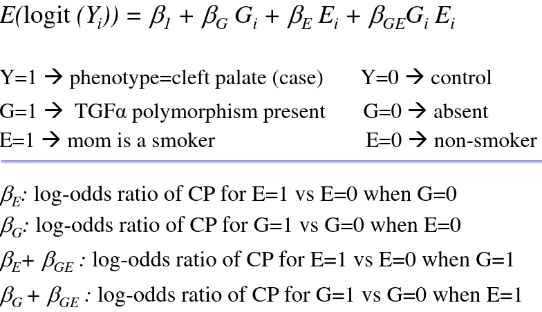

So there are 2 interpretations of β_GE:
1. The difference between the Environment logOR when G = 1 vs when G = 0
2. The difference between the Genotype logOR when E = 1 vs when E = 0

The odds ratio of exposure to non-exposure is exp(beta), or the increased odds of disease at the locus for each additional allele is exp(beta) times smaller for exposure group than non-exposure group.

• Overall we define β_GE is the difference between the observed ln(OR) and the ln(OR) expected when the G and E act additively
  
• When β_GE = 0  (exp(β_GE) = 1):
  • no departure from additivity
  • the genotypic OR in the two groups E = 1 and E = 0 are the same
    
  • the environment odds ratios in the two groups G = 1 and G = 0 are the same

If there is interaction, we should not use summary measures (OR & genotypic means) for the marker or the environmental factor alone. We may improve power to identify genes and SNPs by testing within subgroups of the interacting exposure, or just testing for interaction. 

Detecting Interactions: Power

Even in the GWAS era, there are very few well-known examples of interaction of GxE that have been identified. This is in part due to the fact that tests for interaction are not as powerful as tests for main effect association.

We need much larger sample sizes to detect interaction than main effects, at least 4x the size is needed for same effect. Due to lack of power published reports of GxE interactions may be more prone to publication bias (although usually interaction is not the primary hypothesis in a study). It is better to publish all results to avoid publication bias, but this also leads to many published interactions that have not been replicated.

This power issue is particularly a problem when a large number of markers are tested; as always multiple testing adjustment is required to preserve family-wise error rate. We'll focus on two strategies for maximizing power when conducting GxE GWAS have been proposed: Case-only designs and two-stage screening procedures

Case-Only Design

If G and E are independent (depending on design, in population or among controls) cases from a case-control study can be used to estimate the multiplicative GxE interaction.

When G and E are independent in the controls, the OR for the G-E association among cases equals the multiplicative interaction between E and G. ??Improved precision: acts like a case-control or cohort study with an infinite number of controls.??

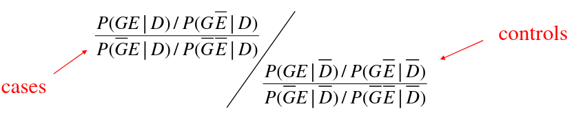
The interaction OR is the ratio of G-E OR in cases to G-E OR in controls. D_bar represents the controls, D represents cases.

If G and E are independent in the controls then the joint probability P(GE | D) = P(G | D)*P(E | D) and the ratio of ORs is just the E-G OR among cases.

We can test for G-E interaction by looking at the G-E association in cases.

Advantages

• Can be inexpensive for exploratory analyses
• Useful for case tissue specimens archived from earlier studies
• Power for the case-only interaction test is much greater than for interaction test in case-control study with same number of cases
• When independence assumption is met, case-only design is much more powerful than case-control logistic regression test of interaction
  

  

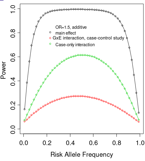
Limitations

• Provides non information about main effects
• The interaction estimate can be biased if the assumption of G-E independence is violated

Two-Stage Screening Procedure

As we've seen GxE tests have poor power compared to the main effect tests, as the multiple testinig problem is more serious. One way to improve power is to do fewer tests, which gives a smaller multiple testing correction and thus larger significance level.

For example, a genome wide test for smoking and SNP interaction power will be very low, as we are usually accounting for > 2.5 million SNPs, so we would need to use a multiple testing correction like alpha = 5x10^-8

Screen procedures are one way to choose which GxE tests to do. A screening procedure gives us a way to select only a small subset of the SNPs m << M to test for G-E interaction. So, we adjust for m SNPs instead of M SNPs, making significance alpha/m instead of alpha/M.

The tricky part is the screening procedure must be independent of the G-E interaction test in order to maintain alpha, also the screening test needs to be good at identifying variants that are likely to have a G-E interaction.

• Stage 1: screen all GWAS SNPs to identify the subset for which there is likely to be a GxE interaction
• Stage 2: Test for interaction only for the m SNPs that passed the stage 1 screening
• Use the same data set for stages 1 and 2, this is different than discovery replication 2 stage design which use independent data sets
• Procedures for screening:
  • Main effect screen - stage 1 screen based on main effects of genotype
    • If the SNP is not associated with the outcome phenotype it does not pass stage 1
  • SNP-E screen - Stage 1 screen based on SNP-E association
    • If the SNP is not associated with E  it does not pass stage 1
    • Appropriate only for case-control samples

Kooperberg LeBlanc Stage 1 (Main G Effect Screening)

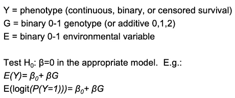
Perform test using all data (E = 0 and E = 1)

• When a GxE interaction exists, except crossover interactions, there will be some evidence of G-Y association in at least some E subgroups(s)
• When the association is strong, it can also be detected marginally in all exposure groups combined
• First stage screening will identify the SNPs more likely to show interaction
• First stage marginal G-Y association test is approximately independent of second-stage interaction test, so significance is preserved
• Most SNPs are not strongly marginally associated with Y so will be removed from consideration of interaction
• Works with cohort data, any phenotype
• Power is lower when the G-Y association is in a different directions in different E strata

Murcray Stage 1 (SNP-E Screening)

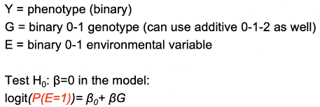
This test is only performed with cases and controls combined.

• If there is no G-E association in the population, interaction exists when there is evidence of G-E association in cases
• When this association is strong, it can also be detected in cases and controls combined
  • Assumes cases are ~1/2 the sample
  • If cases are a small part of of sample, this screen won't work properly (not independent of GxE test)
• Most SNPs will not be associated with E
  • First stage "screening" test will identify SNPs likely to exhibit multiplicative interaction with E on case status
  • First-stage marginal G-R association test is approximately independent of second-stage interaction test, so the significance level for stage 2 corrects only for the stage 2 tests performed

Meta Analysis

GWAS is performed on millions of SNPs. Because of multiple testing, we use very stringent thresholds for statistical significance. This can greatly reduce power and may not be sufficient to detect associated SNPs. Combining information across studies will improve power.

The objective of meta-analysis is to combine results from multiple studies to improve power and get more precise effect estimates.

Limitations of Pooling Raw Data

• May not be possible because of confidentiality restrictions
• May not be desirable because of heterogeneity
  • Differences in population, study design, underlying risk, measurements, etc.

Originally meta-analysis was used to combine results from published studies with small samples to improve power. This is subject to publication bias, only studies with significant p-values are chosen so we are more likely to see a positive effect. Not an issue in GWAS meta-analysis since ALL results are included regardless of significance.

Meta-Analysis of a Single SNP

Collection of K studies to test the same null hypothesis. Each study provides an estimate, beta_hat, of the effect size and a p-value for testing the null hypothesis.

The key assumption is independence of study results, no subjects should appear in more than one study.

The first step in a meta-analysis is to identify a consistent measure from  each study to be summarized (OR, regression coefficient and SE, p-value from chi-square association.

We can use Fisher's method or Stouffer's method, and that's all the information I need for now.