| **Linear Regression** [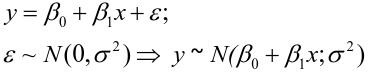](https://bookstack.mitchellhenschel.com/uploads/images/gallery/2022-10/image-1666104229251.png) [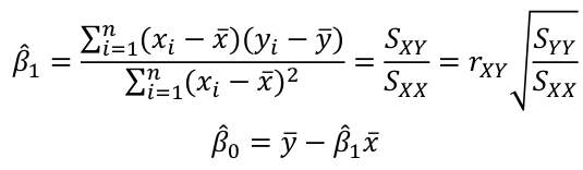](https://bookstack.mitchellhenschel.com/uploads/images/gallery/2022-10/image-1666104239088.png) [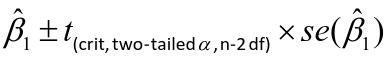](https://bookstack.mitchellhenschel.com/uploads/images/gallery/2022-10/image-1666104245811.png) [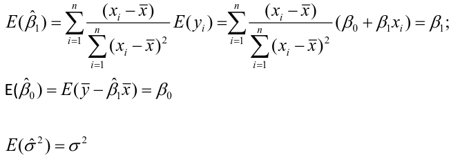](https://bookstack.mitchellhenschel.com/uploads/images/gallery/2022-10/image-1666104252727.png) [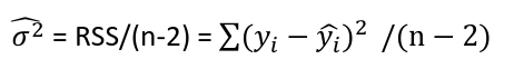](https://bookstack.mitchellhenschel.com/uploads/images/gallery/2022-10/image-1666104260540.png) [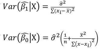](https://bookstack.mitchellhenschel.com/uploads/images/gallery/2022-10/image-1666104271056.png) [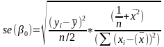](https://bookstack.mitchellhenschel.com/uploads/images/gallery/2022-10/image-1666104276418.png) [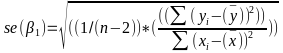](https://bookstack.mitchellhenschel.com/uploads/images/gallery/2022-10/image-1666104282605.png) [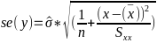](https://bookstack.mitchellhenschel.com/uploads/images/gallery/2022-10/image-1666104287023.png) Predicting a CI new obs adds a 1 to se(y): 𝛽0 + 𝛽2x +/- t\*[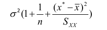](https://bookstack.mitchellhenschel.com/uploads/images/gallery/2022-10/image-1666104297248.png) | **Multiple Linear Regression and Estimation** [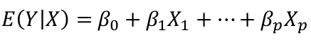](https://bookstack.mitchellhenschel.com/uploads/images/gallery/2022-10/image-1666104323618.png) [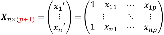](https://bookstack.mitchellhenschel.com/uploads/images/gallery/2022-10/image-1666104327905.png) [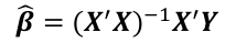](https://bookstack.mitchellhenschel.com/uploads/images/gallery/2022-10/image-1666104332246.png) [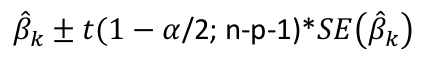](https://bookstack.mitchellhenschel.com/uploads/images/gallery/2022-10/image-1666104336362.png) [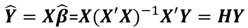](https://bookstack.mitchellhenschel.com/uploads/images/gallery/2022-10/image-1666104345652.png) [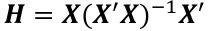](https://bookstack.mitchellhenschel.com/uploads/images/gallery/2022-10/image-1666104350789.png) [](https://bookstack.mitchellhenschel.com/uploads/images/gallery/2022-10/image-1666104355280.png) [](https://bookstack.mitchellhenschel.com/uploads/images/gallery/2022-10/image-1666104359234.png) [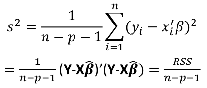](https://bookstack.mitchellhenschel.com/uploads/images/gallery/2022-10/image-1666104363437.png) [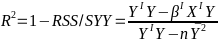](https://bookstack.mitchellhenschel.com/uploads/images/gallery/2022-10/image-1666290673808.png) [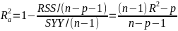](https://bookstack.mitchellhenschel.com/uploads/images/gallery/2022-10/image-1666290691336.png) 𝐻0 : 𝛽1 = 𝛽2 = 𝛽3 = ⋯ = 𝛽𝑝 = 0 v.s. 𝐻1 : not all 𝛽𝑘 = 0, 𝑘 = 1, … , 𝑝 [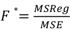](https://bookstack.mitchellhenschel.com/uploads/images/gallery/2022-10/image-1666104389032.png)[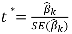](https://bookstack.mitchellhenschel.com/uploads/images/gallery/2022-10/image-1666104395117.png) rejection rule of 𝑡 >= t(1 − alpha/2; 𝑛 − 𝑝 − 1) [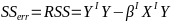](https://bookstack.mitchellhenschel.com/uploads/images/gallery/2022-10/image-1666104407108.png) [](https://bookstack.mitchellhenschel.com/uploads/images/gallery/2022-10/image-1666104410593.png) [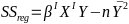](https://bookstack.mitchellhenschel.com/uploads/images/gallery/2022-10/image-1666104415116.png) [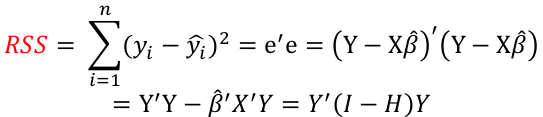](https://bookstack.mitchellhenschel.com/uploads/images/gallery/2022-10/image-1666104423017.png) |
| **Model Fitting: Inference** [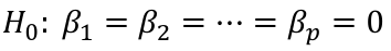](https://bookstack.mitchellhenschel.com/uploads/images/gallery/2022-10/image-1666104576887.png) dfΩ = n - p, and df𝜔 = n – q [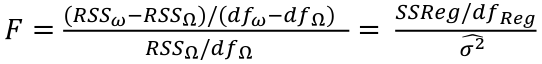](https://bookstack.mitchellhenschel.com/uploads/images/gallery/2022-10/image-1666138531298.png) Reject the null hypothesis if F > Fα p - q, n – p [](https://bookstack.mitchellhenschel.com/uploads/images/gallery/2022-10/image-1666104643517.png) [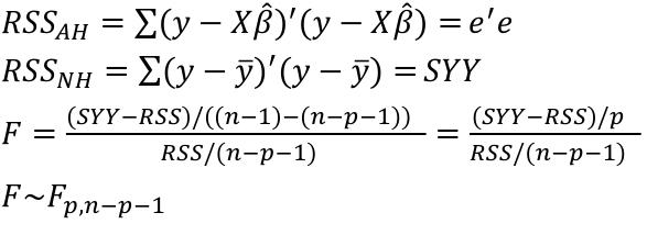](https://bookstack.mitchellhenschel.com/uploads/images/gallery/2022-10/image-1666138340542.png) | **Dummy Variables and Analysis of Covariance** Consider a Xi2 for which is 0 for – and 1 for +: [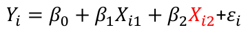](https://bookstack.mitchellhenschel.com/uploads/images/gallery/2022-10/image-1666104607845.png) An interaction between Xi1 and Xi2: [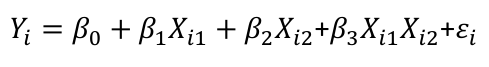](https://bookstack.mitchellhenschel.com/uploads/images/gallery/2022-10/image-1666104615922.png) A model with multiple categorical variables: [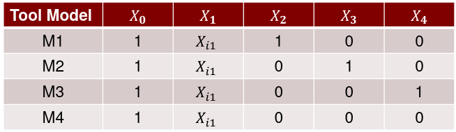](https://bookstack.mitchellhenschel.com/uploads/images/gallery/2022-10/image-1666104625980.png) [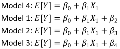](https://bookstack.mitchellhenschel.com/uploads/images/gallery/2022-10/image-1666104633030.png) |
| **Regression Diagnostics** Assumptions: • Error: ~ N(0, SD2I); ◦ Independent ◦ Equal Variance ◦ Normally Distributed • Model: E\[y\] = Xβ is correct • Unusual observations Leverage Points: data point with unusual x-value [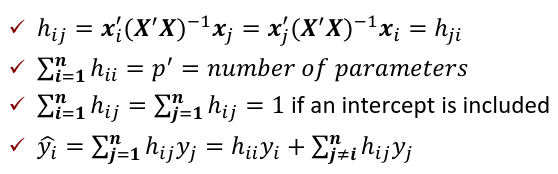](https://bookstack.mitchellhenschel.com/uploads/images/gallery/2022-10/image-1666104773344.png) The Hat Matrix – n\*n matrix hii is the leverage of the ith case leverage > 2p’/n should be looked at closely Outliers: Unusual observation on x or y axis [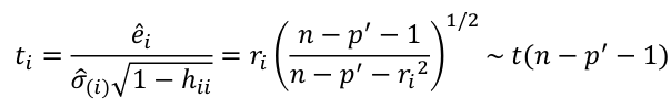](https://bookstack.mitchellhenschel.com/uploads/images/gallery/2022-10/image-1666104790374.png) Calculate the t-test and compare abs with limit: abs(qt(.05/(n\*2), df = n - pprime - 1, lower.tail = T)) | Influential Points: causes changes to regression Difference in Fits: [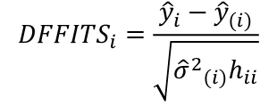](https://bookstack.mitchellhenschel.com/uploads/images/gallery/2022-10/image-1666104815733.png) with a threshold of [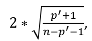](https://bookstack.mitchellhenschel.com/uploads/images/gallery/2022-10/image-1666104825747.png) Where p’ is the number of parameters Cook's Distance: [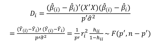](https://bookstack.mitchellhenschel.com/uploads/images/gallery/2022-10/image-1666104834542.png) with a threshold of Di > 4/n should be looked at Di > .5 possible influence Di >= 1 very influential Error: a plot of e\_hat should • have constant variance • have no clear pattern • H0: residuals are normal Shapiro-Wilk normality test H0: Residuals are normally distributed Bonferroni Correction: Divide alpha by n |
| **Variable Selection** Backwards Elimination: 1. Start model with all the predictors 2. Remove the predictor with highest p-value greater than alpha 3. Refit the model 4. Remove the remaining least significant predictor provided its p-value is greater than alpha 5. Repeat 3 and 4 until all "non-significant" predictors are removed Cutoff p significance can be 15-20% for testing Forward Selection: 1. Start model with no predictors 2. For predictors not in the model, check the p-value if they are added to the model. We choose the one with lowest p-value less than alpha 3. Continue until no new predictors can be added Stepwise regression: A combination of the two | Selection Criteria: Akaike Information Criterion (AIC): • -2 max log-likelihood + 2p' • n\*log(RSS/n) + 2p' Bayes Information Criterion (BIC): • -2 max log-likelihood + p' log(n) • n\*log(RSS/n) + log(n) \* p' Adjusted R2: R2 = 1 – RSS/SSY [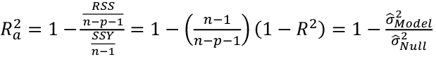](https://bookstack.mitchellhenschel.com/uploads/images/gallery/2022-10/image-1666202623504.png) Mallow’s Cp Statistic: Avg MSE of prediction [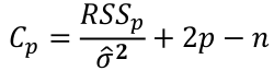](https://bookstack.mitchellhenschel.com/uploads/images/gallery/2022-10/image-1666202639730.png)If a p-predictor fits then: [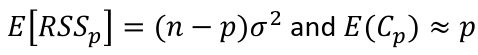](https://bookstack.mitchellhenschel.com/uploads/images/gallery/2022-10/image-1666202661358.png) We desire models with small p and Cp around or less than p |
| \# Model with only beta\_0 sr\_lm0 <- lm(y ~ 1, data=sr) \# Full model sr\_lm1 <- lm(y ~ ., data=sr) sr\_syy <- sum((savings$sr - mean(savings$sr))^2) sr\_rss <- deviance(sr\_lm1) \# F = ((SYY -RSS)/((n-1) - (n-2))) / (RSS / (n - 1)) sr\_num <- (sr\_syy - sr\_rss)/(df.residual(sr\_lm0) - df.residual(sr\_lm1)) sr\_den <- sr\_rss / df.residual(sr\_lm1) sr\_f <- sr\_num / sr\_den \# dfΩ = n - p, and df𝜔 = n - q pf(sr\_f, df.residual(sr\_lm0) - df.residual(sr\_lm1), df.residual(sr\_lm1), lower.tail = F) \# β=(XI X)−1 XIY beta <- solve(t(x)%\*%x)%\*%(t(x)%\*%y) \# Pearson's cor(lin\_reg$fitted.values, lin\_reg$residuals, method="pearson") \# Stratify variables by a factor by(depress, depress$publicassist, summary) \# Welsh's Two Sample T-test \# For difference in means t.test(assist$cesd, noassist$cesd) \# or t.test(data.y ~ factor) \# CI of LS means based on covariates library(lsmeans) lsmeans(reg, ~Type) \# Apply a mean function to an array \# split on a factor tapply(assist$cesd, assist$assist, mean) \# When a regression factor has \# more than two categories reg <- lm(Pulse1 ~ Height + Sex + Smokes + as.factor(Exercise)) | \# Cook's Distance cook <- cooks.distance(reg) cook\[cook > 4/n\] \# Shapiro Test for normallity shapiro.test(reg$residuals) \# Studentized residuals stud <- rstudent(reg) \# Threshold for lower tail of \# studentized resids with correction lim = abs(qt(.05/(n\*2), df = n - pprime - 1, lower.tail = T)) stud\[which(abs(stud) > lim)\] \# Hat values hat <- hatvalues(reg) lev <- 2 \* pprime / n hat\[hat > lev\] \# Forward selection forward <- ~ year + unemployed + femlab + marriage + birth + military m0 <- lm(divorce ~ 1, data = usa) reg.forward.AIC <- step(m0, scope = forward, direction = "forward", k = 2) n <- nrow(usa) \# AIC = n\*log(RSS/n) + 2p' n\*log(162.1228/n)+2\*6 extractAIC(reg.forward.AIC, k=2) \# BIC reg.forward.BIC <- step(m0, scope = forward, direction = "forward", k = log(n)) extractAIC(reg.forward,k=log(n)) \# BIC = n\*log(RSS/n) + p'\*log\*n) n\*log(162.1228/n)+6\*log(n) library(leaps) leaps <- regsubsets(divorce ~ .) rs <- summary(leaps) par(mfrow=c(1,2)) plot(2:7, rs$cp, xlab="No. of parameters", ylab="Cp Statistic") abline(0,1) |
In R the 'prcomp()' function computes principal components by using a **singular value decomposition.**
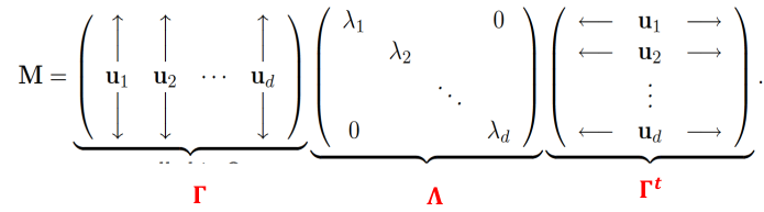
The advantage of using PCA is that we hope to end up with a number of components that is smaller than the number of variables p. We can use PCA for data reduction techniques. If 2 or 3 PCs explain a large portion of the total variance, then we can use these 2 or 3 variables for analysis rather than the whole set. ## Spectral Decomposition The spectral decomposition recasts a matrixx in terms of it eignenvalues and eigenvectors. The representation turns out to be very useful.Let M be a real **symmetric** d x d matrix with eigen values lambda\_1, lambda\_2, ..., lambda\_d and corresoinding orthonormal eigenvectors u1, u2, ..., ud then:
[](https://bookstack.mitchellhenschel.com/uploads/images/gallery/2022-11/image-1667516527816.png) ## R Code ``` ### Example 1 head(USArrests) dim(USArrests) sqrt(apply(USArrests,2,var)) plot(USArrests) # compute principal components pca1 <- prcomp(USArrests, scale=T) pca1 (13.2 -mean(USArrests$Murder))/sqrt(var(USArrests$Murder))*( -0.5358995) + (236-mean(USArrests$Assault))/sqrt(var(USArrests$Assault))*(-0.5831836) + (58-mean(USArrests$UrbanPop))/sqrt(var(USArrests$UrbanPop))*(-0.2781909) + (21.2-mean(USArrests$Rape))/sqrt(var(USArrests$Rape))*(-0.5434321) sum(((USArrests[1,]-pca1$center)/pca1$scale)*pca1$rotation[,1]) ## generate summary of loadings summary(pca1) plot(pca1) # extract principal components pca1$x[1:5,] # plot PCs plot(pca1$x[,1:2]) biplot(pca1) ``` # Intro to Cluster Analysis **Clutsering** refers to a very broad set of techniques for finding subgroups, or clusters, in a data set. When we cluster the observations, we partition the profiles into distinct groups so that the profiles are similar within the groups but different from other groups. To do this, we must define what makes observations similar or different. ##### PCA vs Clustering Both clustering and PCA seek to simplify the data via a small number of summaries, but their mechanisms are different: - PCA searches for a low-dimensional representation of the observations that explains a good fraction of the variance - Clustering looks to find homogeneous subgroup among the observations ##### Notation Input is data with p variables and n subjects [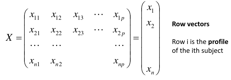](https://bookstack.mitchellhenschel.com/uploads/images/gallery/2022-11/image-1668562361706.png) A distance between two vectors i and j must obey several rules: - The distance must be positive definite, dij >= 0 - The distance must be symmetric, dij = dij, so that the distance from j to i is the same as the distance from i to j - An object is zero distance from itself, dii = 0 - The triangle rule - When considering three objects i, j and k the distance from i to k is always less than or equal to the sum of the distance from i to j and the distance from j to k dik <= dij + djk #### Clustering Procedures - **Hierarchical clustering**: Iteratively merges profiles into clusters using a simple search. Start with each profile/cluster and end with one 1. The clustering procedure is represented by a *dendrogram*. - **K-mean clustering:** Start with a per-specified number of clusters and random allocation of profiles to clusters. Iteratively move profiles from one cluster to the other to optimize some criterion. End up with the same number of clusters. ### K-Means Clustering We partition the K clusters so that we maximize the similarity within clusters and minimize the similarity between clusters. We can represent the data with a vector of means, which is the overall profile or cluster: [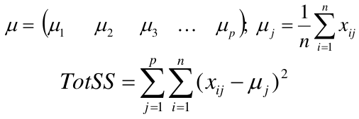](https://bookstack.mitchellhenschel.com/uploads/images/gallery/2022-11/image-1668606369350.png) Supposed we split the data into 2 clusters, C1 with 𝑛1 observations of the p variables, and C2 with 𝑛2 observations of the p variables. We would have two different vectors of means representing the centroids of the clusters. The total sum of squares within clusters would be: [](https://bookstack.mitchellhenschel.com/uploads/images/gallery/2022-11/image-1668606548035.png) And we seek to keep WSS small, but it is NOT guaranteed to give the minimum WSS so ideally one should start from different initial values. - Start with K "random" clusters by assigning each of the n profiles to one of the K clusters at random - Iterate until no more changes are possible: - For each of the K clusters, compute the cluster profile (centroid) - Assign each observation to the cluster whose centroid is closest (using Euclidean distance) [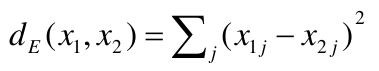](https://bookstack.mitchellhenschel.com/uploads/images/gallery/2022-11/image-1668606130150.png) Example with K = 3, p = 2: [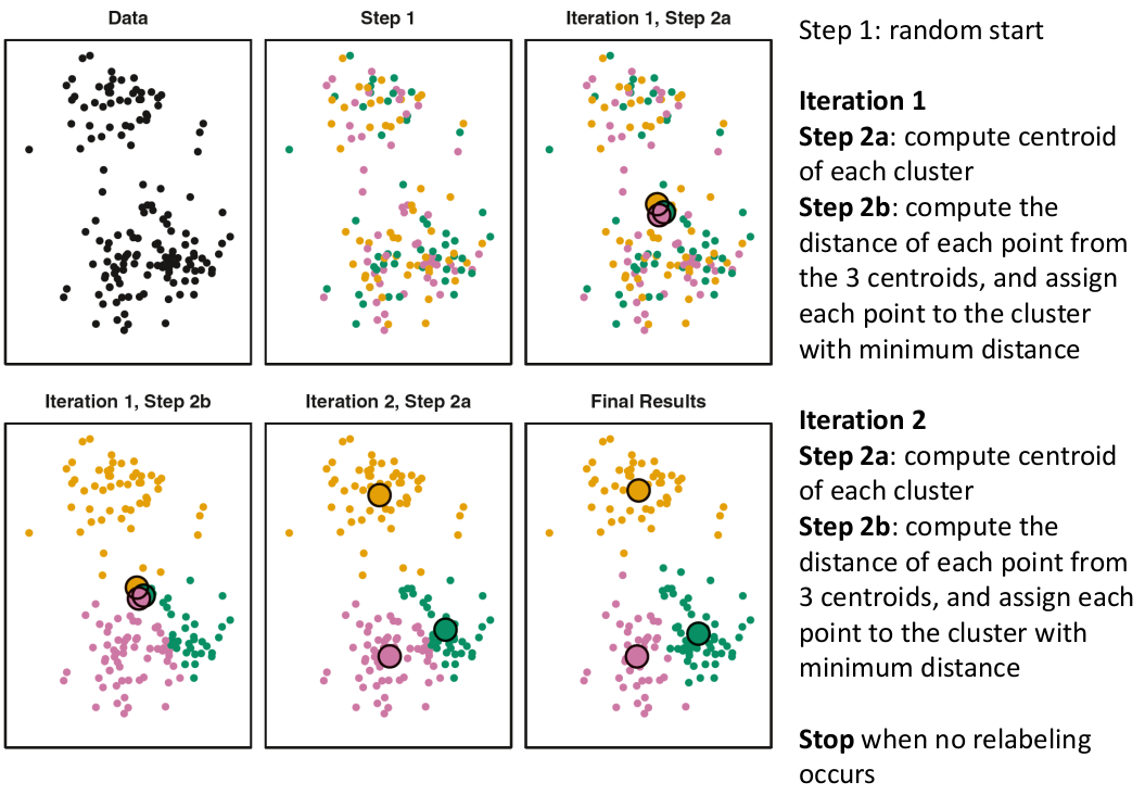](https://bookstack.mitchellhenschel.com/uploads/images/gallery/2022-11/image-1668607255893.png) #### Standardization When the variables are measured on different scales the measurement units may bias the cluster analysis. The Euclidean distance is not scale invariant. ### Hierarchical Clustering This is an alternative approach that does not require a fixed number of clusters. The algorithm essentially rearranges profiles so that similar profiles are displayed next to each other in a tree (dendrogram) and the dissimilar profiles are displayed in different branches. [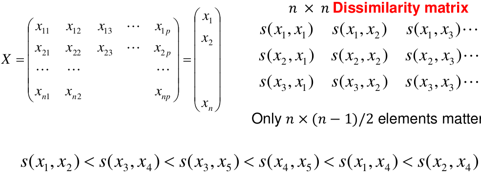](https://bookstack.mitchellhenschel.com/uploads/images/gallery/2022-11/image-1668611245622.png) [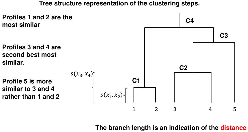](https://bookstack.mitchellhenschel.com/uploads/images/gallery/2022-11/image-1668611376451.png) We do this we define the similarity (distance) between: - Two profiles: s(xi, xi) - A profile and a cluster: s(xc, xi) - Two clusters: s(xc, xc) #### Similarity Between Clusters ##### Complete-Linkage Clustering - Also known as the maximum or furthest-neighbor method - The distance between two clusters is calculated as the greatest distance between members of the relevant clusters - This method tends to produce very compact clusters of elements and the clusters are often similar in size ##### Single-Linkage Clustering - Referred to as the minimum or nearest neighbor method - The distance between two clusters is calculated as the minimum distance between members of the relevant clusters - This method tends to produce clusters that are 'loose' because clusters can be joined if any two members are close together. In particular, this method often results in 'chaining' or sequential addition of single samples to an existing cluster and produces trees with many long, single-addition branches. ##### Average-Linkage Clustering - The distance between clusters is calculated using average values. There are various methods used for calculating this average. The most common is the unweighted pair-group method average (UPGMA), where each average is calculated from the distance between each point in a cluster and all other points in another cluster and the 2 clusters with the lowest average distance are joined together into a new cluster. ##### Centroid Clustering - Related methods substitute the centroid for the average. **Complete and average linkage are similar, but complete linkage is faster because it does not require recalculation of the similarity matrix at each step.** [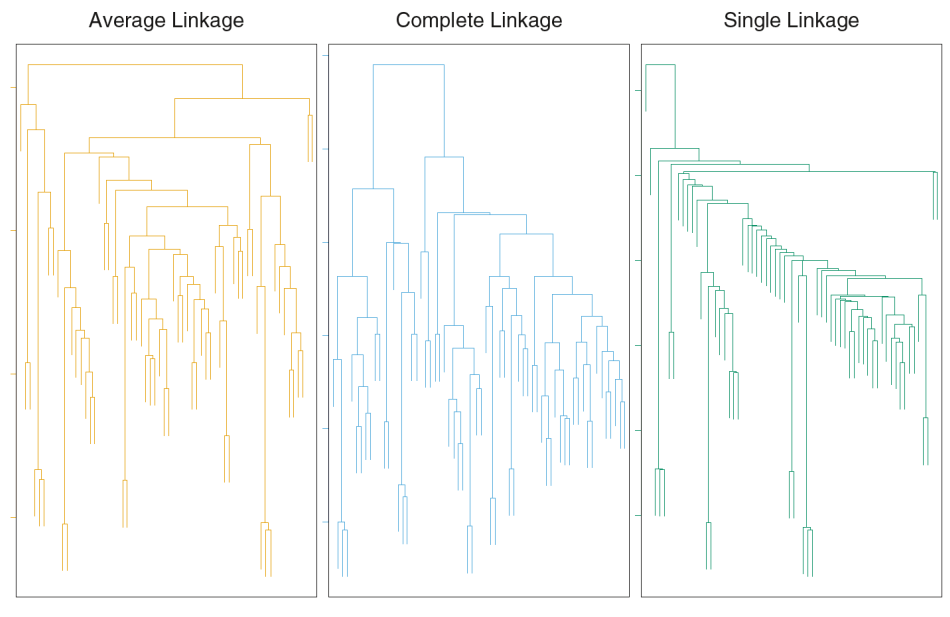](https://bookstack.mitchellhenschel.com/uploads/images/gallery/2022-11/image-1668612158830.png) ### Detection of Clusters Inspection of the QQ-plot would inform about the existence of clusters in the data. [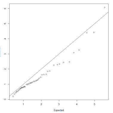](https://bookstack.mitchellhenschel.com/uploads/images/gallery/2022-11/image-1668612379283.png) - Observed and “expected” distances are statistically indistinguishable would suggest that there are no clusters in the data - Departure of the QQ-plot from the diagonal line would suggest that there are clusters We can also use a 95%-tile to detect the number of clusters using extreme percentiles of the reference distribution. The idea is to color the entry of the data set, so that the colors represent the standardized difference of the cell intensity from a baseline. Typically, columns are samples and rows are variables. [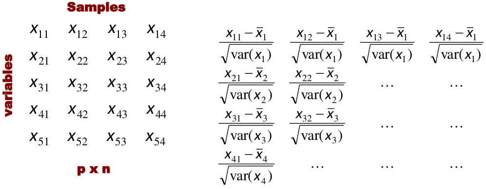](https://bookstack.mitchellhenschel.com/uploads/images/gallery/2022-11/image-1668612715262.png) [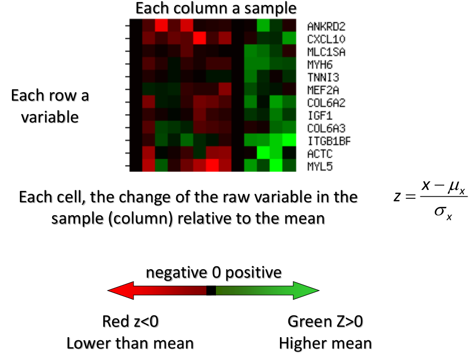](https://bookstack.mitchellhenschel.com/uploads/images/gallery/2022-11/image-1668612745091.png) # Classification **Classification** is often used to describe modeling of a categorical outcome. In binary classification the outcome is two possible values/classes and the goal is the predict the correct class using covariates. **Classification rule:** A mathematical function to predict the outcome of a new sample unit when the values of the covariates are known. ##### Common Classification Problems - Molecular diagnostic: Using values of gene products (such as biomarkers) develops a diagnostic tool for early detection of diseases. - Classification of cancer type: Different sub-types of cancer are characterized by a combination of specific markers that are on/off. Gene based classification rules can be used to increase the specificity of the diagnosis. - Classification of drug response - Risk prediction #### Types of Classifiers - Regression-based: - Logistic regression, CART - Example-based: - KNN - Based on Bayes theorem: - Discriminant analysis - Ensemble of classifiers To evaluate a classifier, split the data into a training and test set. Use the training set to build the classification rule and the test set to evaluate how the classification rule labels new cases with known label. ### Logistic Regression [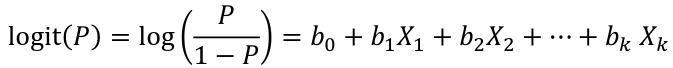](https://bookstack.mitchellhenschel.com/uploads/images/gallery/2022-11/image-1668726889867.png) bi, i = 0,1... k can be estimated using Maximum Likelihood To estimate the probability of a binary outcome as a function of covariates with logistic regression:[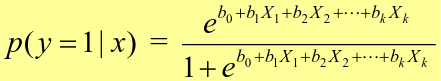](https://bookstack.mitchellhenschel.com/uploads/images/gallery/2022-11/image-1668727009638.png) ##### How to Pick Classification Rule We can use the above formula for x in \[0,1\] to generate thresholds based on the predicted value to decide how to classify. Accuracy is the rate of correctly classified labels in the test set: [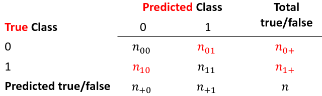](https://bookstack.mitchellhenschel.com/uploads/images/gallery/2022-11/image-1668727368514.png) Misclassification error: False positive: prediction 1 and true is 0; n01 / n0+ False negative: predict 0 and true is 1; Fn10 / n1+ Accuracy: (n00 + n11) / (n00 + n01 + n10 + n11) Sensitivity (recall) the metric of true positive detection and shows whether the rule is sensitive to identify positive outcomes: 1 - n10 / n1+ = n11/n1+ = 1 - FNR Specificity is the measure of true negative detection and shows whether the rule is specific in detection of negative outcomes: 1 - n01 / n0+ = n00 / n0+ = 1 - FPR You CANNOT maximize sensitivity and specificity simultaneously. Maximum sensitivity test always says 1, maximum sensitivity always says 0. Positive/Negative predicted values: The number of correct all predicted positive/negative values #### ROC (Receiver Operating Characteristics) Analysis The ROC curve is a population graphic for simultaneously displaying the two types of errors for all possible thresholds. They are useful for comparing different classifiers since they take into account all possible thresholds. The overall performance of a classifier, summarized over all possible thresholds is given by the area under the ROC curve (AUC). An ideal ROC curve will hug the top-left corner, so the larger the AUC the better the classifier. We expect a classifier that performs no better than chance to have an AUC of .5 #### Steps to Build and Evaluate Classification Rule: 1. Generate training and test set 2. Generate the classification rule using the training set; 3. Generate the predicted rules in the test set; 4. Use ROC analysis to decide the threshold that gives a good balance between sensitivity and specificity. 5. The next examples will show a variety of methods to generate classification rules (so step 2) The previous chapter describes methods to create classification trees and K-nearest neighbor. #### Discriminant Analysis Logistic regression involves directly modeling P(Y = k | X = x) using logistic function. An alternative approach will model the distribution of the predictors X separately in each of the response classes, then use Bayes theorem to flip these around into estimates for P(Y = k | X =x) Assuming the covariate x is normally distributed: [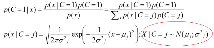](https://bookstack.mitchellhenschel.com/uploads/images/gallery/2022-11/image-1668730683857.png) Binary outcome: Classify as 1 if p(C = 1 | x) > p(C = 0 | x) [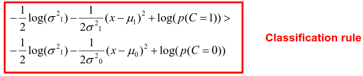](https://bookstack.mitchellhenschel.com/uploads/images/gallery/2022-11/image-1668730751004.png) A special case when the variances of X in the groups are the same: [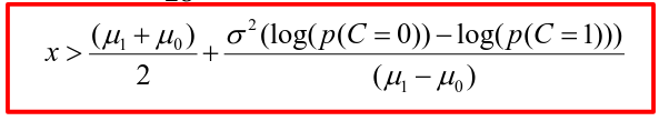](https://bookstack.mitchellhenschel.com/uploads/images/gallery/2022-11/image-1668730805144.png) #### More than One Feature To extend this approach to multiple covariates, one needs to decide: 1. How to model the correlation of the covariates within each group defined by the outcome 2. If the correlation of the covariates changes in different groups LDA - assumes equal variance-covariance structure between groups QDA - assumes group specific variance covariance matrices LDA/QDA models all covariates as normal distributions ### Summary For each method: 1. Fit the classification model using training data 2. Evaluate the classification accuracy in test data using ROC analysis 3. Can also choose a “best” threshold to optimize sensitivity/specificity 4. Compare different classifiers by their AUC The final classifier should be trained on all data to be used for future applications There is no single "Best Classification Method". There is clear evidence that different methods work better in some data and worse in others. Thus, we often use the prediction probabilies of various classifiers to build an ensemble, using prediction probabilities from various rules. This is limited as there is no description of mechanism, useful only for prediction. # Two-Way ANOVA We've learned about One-Way Analysis of Variance (ANOVA) previously, it is a regression model for one continuous outcome and one categorical variable. It allows us to compare the means of the groups to detect significant differences. A one-way fixed-effects ANOVA is an extension of the two-sample t-test. There are **factors**, categorical variables, and **levels**, individual groups of the factor which represent different populations. Balanced design contain the same number of individuals in each level. **This is a special case of linear regression.** Assumptions of one-way ANOVA: - The data are random samples from k independent populations - Within each population the dependent variable is normally distributed - The observations are independent - The population variance of the dependent variable is equal in all groups (homoscedasticity)H0: The mean level is independent of the factor
Ex. The mean testosterone level is independent of smoking history. A conclusion might be "there is evidence that testosterone level is significantly different in at least two of the smoking history groups. We test the hypothesis by decomposing the overall variance into "explained" and "residual" variances and comparing them. [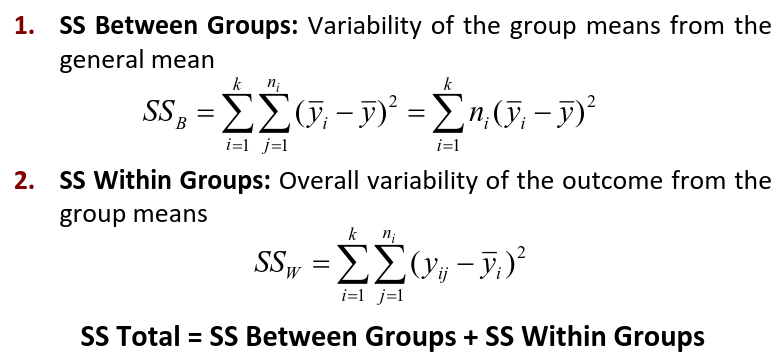](https://bookstack.mitchellhenschel.com/uploads/images/gallery/2022-12/image-1669936903897.png) Where N is the total sample size and k is the number of groups SSB represents the variability due to the treatment effect. SSW represents the residual variability. [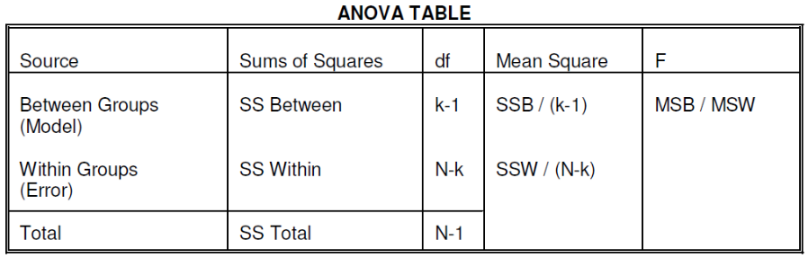](https://bookstack.mitchellhenschel.com/uploads/images/gallery/2022-12/image-1669937073680.png) We compare the F statistic to the critical value of F with \[(k - 1), (N - k)\] degrees of freedom to test the null hypothesis of equal means. #### Multiple Comparisons Procedures To find which means are different from each other we should make all pairwise comparisons (k\*(k-1)/2). This introduces the multiple tests issues and increases likeliness of type I and II errors. Multiple comparison procedures take into account the total number of comparisons being made by lowering the significance level for each test so that the overall significance level is still fixed at some level alpha. [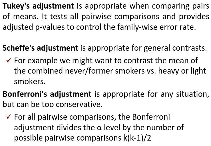](https://bookstack.mitchellhenschel.com/uploads/images/gallery/2022-12/image-1669937488081.png) All of these adjustments are appropriate when comparing pairs of means. Tukey's is the most powerful and provides exact p-values when the group sizes are equal. Scheffe's procedure is more powerful than Bonferroni's procedure, in general. We can also write ANOVA as a linear regression model where **the parameter alpha\_i are the group effects** (difference of effect between group i and group 1) ### Two Way ANOVA Two way ANOVA is a regression model for one continuous outcome and **two** categorical variables. We analyze two-way ANOVA experiments using additive and interaction models. Critical assumptions: - Observations at different factor levels are samples from normal distributions - The variances of the different populations are the same An experiment may also contain replication, for example consider the following tables: [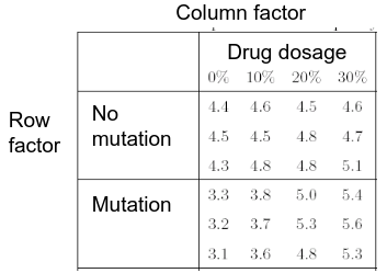](https://bookstack.mitchellhenschel.com/uploads/images/gallery/2022-12/image-1669938856486.png)[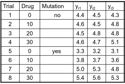](https://bookstack.mitchellhenschel.com/uploads/images/gallery/2022-12/image-1669939027651.png) Both are the same data where the two factors are drug dosage and mutation, and we have 3 replications. We can create summaries of the means: [](https://bookstack.mitchellhenschel.com/uploads/images/gallery/2022-12/image-1669938936434.png) [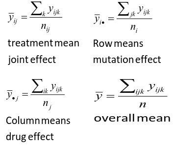](https://bookstack.mitchellhenschel.com/uploads/images/gallery/2022-12/image-1669938962004.png) ##### Possible Models **Interaction model**: The effect of each factor changes as the other factor levels vary [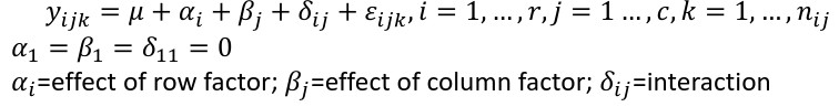](https://bookstack.mitchellhenschel.com/uploads/images/gallery/2022-12/image-1669938523361.png) **Additive** **model**: The effect of each factor doesn't change as the other factor levels vary [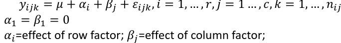](https://bookstack.mitchellhenschel.com/uploads/images/gallery/2022-12/image-1669938550315.png) We test different models using ANOVA to look at the global effect of the factors #### Sum of Squares The traditional one-way ANOVA uses a decomposition of the sum of squares for analysis. [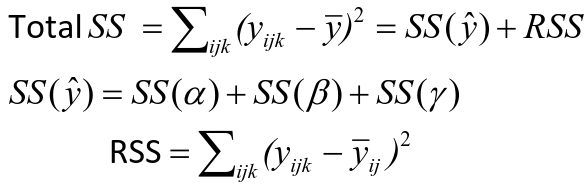](https://bookstack.mitchellhenschel.com/uploads/images/gallery/2022-12/image-1669939467503.png) Each sum of squares uses a number of degrees of freedom, given by number of different levels - 1 [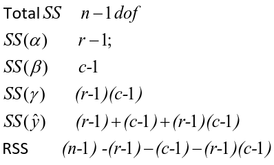](https://bookstack.mitchellhenschel.com/uploads/images/gallery/2022-12/image-1669939431751.png) [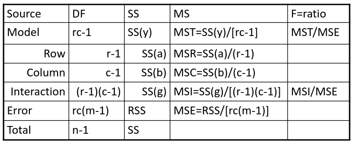](https://bookstack.mitchellhenschel.com/uploads/images/gallery/2022-12/image-1669939548755.png) SS(y) = model SS = SS(a) + SS(b) + SS(g) These sum of squares are computed sequentially, so **the order of terms in the model matters**! If the design is balances the order does not matter. #### Steps 1. Goodness of fit/Global null hypothesis H0: All parameters = 0 Ha: At least one differs from 0 2. Test interaction - F test is MSI/MSE ~ F(r-1)(c-1), rc(m-1) - The P-value is p(F(r-1)(c-1), rc(m-1) > F | H0) - If the p-value is smaller than our alpha then we reject the null - If we do not reject the null, there is no evidence that all interaction terms are not 0. Fit an additive model and repeat 3. Test main effects - If we accept the null hypothesis of no interaction, it makes sense to test the significance of the main effects, to do this we pool the RSS with SS(y) - SS(a) and SS(b) are Type III sum of sqaures Once a model is accepted one can do mean comparisions to identify the factor levels with different effects (Tukey's). The balance design means the the design is orthogonal and so there is no need to recompute sum of squares or estimates for different models. If not, analyze the data as a traditional linear model. #### Problems When the design is orthogonal/balanced the decomposition SS(a) + SS(b) + SS(g) is unique, when it is not the decomposition depends on the order. [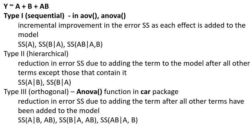](https://bookstack.mitchellhenschel.com/uploads/images/gallery/2022-12/image-1669941015789.png) ## R Code ``` ####### Two-way ANOVA ##### drug dataset drug <- read.csv("anova.csv", header=T) drug hbf <- c(t(drug[,3:5])) SNP <- c(rep("No",12), rep("Yes", 12)) Drug <- c(rep(0,3), rep(10,3), rep(20,3), rep(30,3), rep(0,3), rep(10,3), rep(20,3), rep(30,3)) data.drug <- data.frame(hbf,SNP, Drug) head(data.drug) ### summaries overall.mean <- mean(hbf); overall.mean drug.means <- tapply(hbf, Drug, mean); drug.means snps.means <- tapply(hbf, SNP, mean); snps.means cell.means <- tapply(hbf, interaction(Drug,SNP), mean); cell.means dim(cell.means) <- c(4,2); cell.means cell.means <- data.frame(cell.means) row.names(cell.means) <- levels(factor(Drug)) names(cell.means) <- levels(factor(SNP)) cell.means ## Visualization #install.packages("gplots") library(gplots) plotmeans(hbf~Drug, data=data.drug,xlab="Drug", ylab="HbF", main="Mean Plot\n with 95% CI") plotmeans(hbf~SNP, data=data.drug,xlab="SNP", ylab="HbF", main="Mean Plot\n with 95% CI") plotmeans(hbf~interaction(Drug,SNP), data=data.drug, xlab="SNP", connect=list(1:4,5:8),ylab="HbF", main="Interaction Plot\nwith 95% CI") interaction.plot(factor(Drug), factor(SNP), hbf, type="b", xlab="Drug", ylab="hbf", main="Interaction Plot") ### two-way anova with balanced design mod <- aov(hbf~as.factor(Drug)*SNP, data=data.drug) summary(mod) table(mod$fitted.values) # TukeyHSD(mod) mod <- lm(hbf~as.factor(Drug)*SNP, data=data.drug) summary(mod) anova(mod) table(mod$fitted.values) ##### Exercise with balance design mod.a <- aov(hbf~as.factor(Drug)*SNP, data=data.drug) summary(mod.a) # anova(mod.a) mod.lma <- lm(hbf~as.factor(Drug)*SNP, data=data.drug) anova(mod.lma) mod.b <- aov(hbf~SNP*as.factor(Drug), data=data.drug) summary(mod.b) # anova(mod.b) mod.lmb <- lm(hbf~SNP*as.factor(Drug), data=data.drug) anova(mod.lmb) ##### Exercise with unbalance design data.drug.1 <- read.csv("data.drug.1.csv", header=T) mod.1a <- aov(hbf~as.factor(Drug)*SNP, data=data.drug.1) summary(mod.1a) mod.1lma <- lm(hbf~as.factor(Drug)*SNP, data=data.drug.1) anova(mod.1lma) mod.1b <- aov(hbf~SNP*as.factor(Drug), data=data.drug.1) summary(mod.1b) mod.1lmb <- lm(hbf~SNP*as.factor(Drug), data=data.drug.1) anova(mod.1lmb) ```