Multivariable Analysis

• Simple Linear Regression
• Mutiple Linear Regression and Estimation
• Model Fitting: Inference
• Dummy Variables and Analysis of Covariance
• Broken Stick Regression, Polynomial Regression, Splines
• Regression Diagnostics
• Variable Selection
• Midterm Cheat Sheet
• Tree Based Methods
• Principal Component Analysis
• Intro to Cluster Analysis
• Classification
• Two-Way ANOVA

Simple Linear Regression

One of the first known uses of regression was to study inheritance of traits from generation to generation in a study in the UK from 1893-1898. E.S. Pearson organized the collection of heights of mothers and one of their adult daughters over 18. The mother's height was the predictor variable (x) and the daughter's height was the response variable (y).

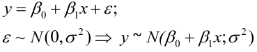
The goal of a linear regression is to quantify the relationship between one independent variable and a single dependent variable. A simple linear regression can be represented by the following:

• y_hat = β₀ + β₁x + Error; E(Error) = 0; V(Error) = σ²
• E(y) = β₀ + β₁x ; V(y) = σ²
  

As with correlation, a strong association in a regression analysis does NOT imply causality

Additionally, prediction values outside the range of values observed for x is not reliable, and is called extrapolation.

Least Squares Estimation

OLS/LS - Ordinary Least Squares is a method that looks for the line that minimizes the "residual sum of squares"

    Residual = Observed - Predicted = y - ŷ

So we can set up an equation for sum of squared residuals:    ∑(y - ŷ)²

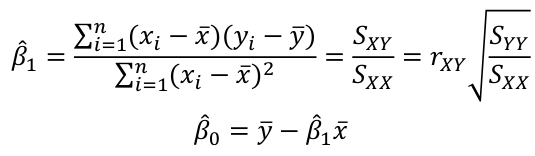
Then substitute  the linear regression equation, take the derivative, set to zero and solve.The solution comes out to:

The fitted equation will pass through x bar, y bar (the center of data)

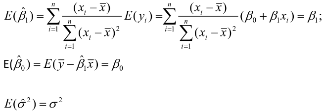
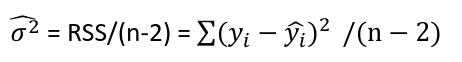
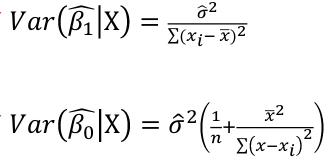
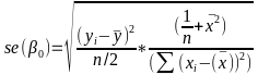
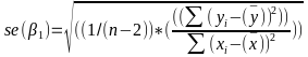
Estimating Variances of LSE

The square root of an estimated variance is called standard error represented by s or se().

E(Y |X = x) = a function that depends on the value of x

LSE Assuming Normally Distributed Data

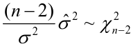
The distributions of estimates are used to make predictions and hypothesis testing. Since variance of a fixed variable is 0, we can estimate the error of a normal distribution as follows:

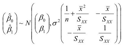
The estimates are correlated with covariance -x_bar/S_xx

It can be shown that the Least Squares Estimate is also the Maximum Likelihood Estimate.

Confidence Intervals

The distribution of β₁ is normal if the variance is known.

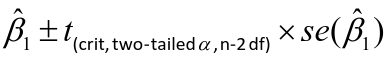
When we use estimated variance, we use a Student's t distribution on n-2 degrees of freedom to estimate parameters:

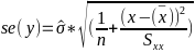
By finding the standard error of y_hat we can also calculate a confidence interval for a fitted value, or a given of x

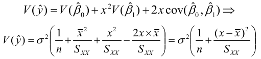
The interval width is:

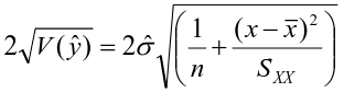
And width will increase as the distance between observed and expected increases.

ANOVA

Though ANOVA is usually used in determining if there is a difference in variance with data containing 3 or more categories, linear regression under standard conditions is a special case of ANOVA. The name analysis of variance is derived from a partitioning of total variability into its component parts.

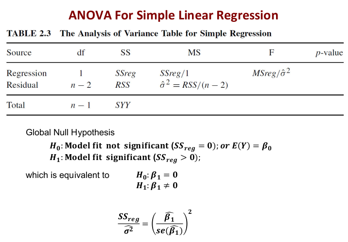
This formula uses an F-distribution with 1 and n − 2 df in place of the t-distribution to correct for the simultaneous inference from our estimate of Beta_1.

Prediction of New Observations

When using points not in the dataset (extrapolation) use the following adjusted formulas for variance of V(y):

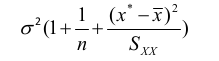
Thus, the confidence interval for a new observation would be significantly wider

Other notations commonly seen in our textbook

Mutiple Linear Regression and Estimation

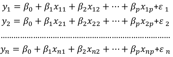
Multiple Linear Regression analysis can be looked upon as an extension of simple linear regression analysis to the situation in which more than one independent variables must be considered.

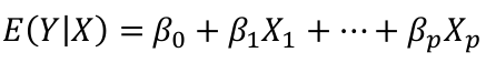
The general model with response Y and regressors X₁, X₂,... X_p:

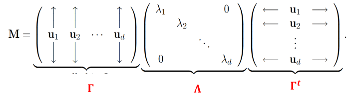
Suppose we observe data for n subjects with p variables. The data might be presented in a matrix or table like:

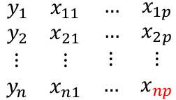
We could then write the model as:

We can think of Y and E as (n x 1) vectors when transposed, and β as a ((p + 1) x 1) vector.  p +1 is number of predictors + the intercept. Thus X would be:

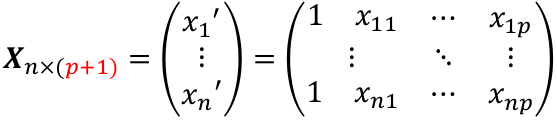
The general linear regression may be written as:

Or     y_i = x_i^|*β + ∈_i

The model is represented as the systematic structure plus the random variation with n dimensions = (p + 1) + { n - (p + 1 ) }

Ordinal Least Squares Estimators

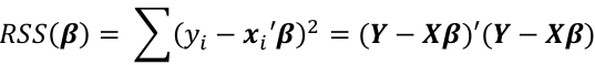
The least squares estimate β_hat of β is chosen by minimizing the residual sum of squares function:

By differentiating with respect to β_i and solve by setting equal to 0:

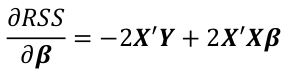
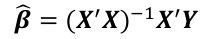
The least squares estimate of β_hat of β is given by: 

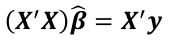
and if the inverse exists:

Fitted Values and Residuals

The fitted values are represetned by Y_hat = X*β_hat

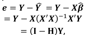
where the hat matrix is defined as H = X(X^|X)^-1X^|

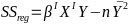
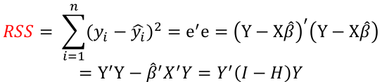
The residual sum of squares (RSS): 

Gauss-Markov Conditions

In order for estimates of β to have some desirable statistical properties, we need a set of assumptions referred to as the Gauss-Markov conditions; for all i, j = 1... n

1. E[∈_i] = 0
2. E[∈_i²] = 𝜎²
3. E[∈_i∈_j] = 0, where i != j

Or we can write these in matrix notation as:  E[∈] = 0, E[∈∈^|] = 𝜎²*I

The GM conditions imply that E[Y] = Xβ and cov(Y) = E[(Y-Xβ)(Y-Xβ)^|] = E[∈∈^|] = ∈

Under the GM assumptions, the LSE are the Best Linear Unbiased Estimators (BLUE). In this expression, "best" means minimum variance and linear indicates that the estimators are linear functions of y.

The LSE is a good choice but it does require the errors are uncorrelated and have equal variance. Even if the errors behave, then nonlinear or biased estimates may work better.

Estimating Variance

By definition:

We can estimate variance by an average from the sample:

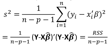
Under GM conditions, s² is an unbiased estimate of variance.

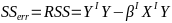
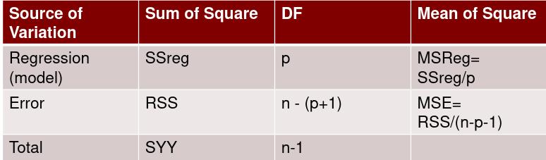
Total Sum of Squares

Total sum of squares is Syy = SSreg + RSS

The corrected total sum of squares with n-1 degrees of freedom:

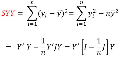
where J is an n x n matrix of 1s and H = X(X^|X)^-1X^|

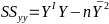
Regression and Residual Sum of Sqaures

Regression sum of squares represent the number of X variables:

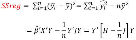
Residual Sum of Squares with n - (p + 1) degrees of freedom:

F Test for Regression Relation

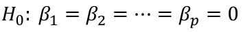
To test whether there is a regression relation between Y and a set of variables X, use the hypothesis test:

𝐻0 : 𝛽1 = 𝛽2 = 𝛽3 = ⋯ = 𝛽𝑝 = 0  v.s.  𝐻1 : not all 𝛽𝑘 = 0, 𝑘 = 1, … , 𝑝

We use the test statistic:

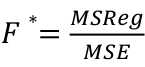
The chances of a Type I error is alpha, our degrees of freedom is n - p -1

The Coefficient of Determination

Recall this measures the model of fit by the proportionate reduction of total variation in Y associated with the use of the set of X variables.

R² = SSreg / Syy = 1 - RSS / Syy

In a multi-linear regression we must adjust the coefficient by the associated degrees of freedom:

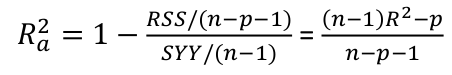
Add more independent variables to the model can only increase R², but R²_alpha may become smaller when more independent variables are introduced, as the decrease in RSS may be offset by the loss of degrees of freedom.

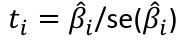
T Tests and Intervals

Tests for β_k are pretty standard:

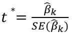
With the rejection rule of 𝑡 >= t(1 − 𝛼/2; 𝑛 − 𝑝 − 1)

And likewise confidence limits for β_k and 1 - alpha confidence

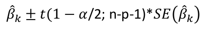
Model Fitting: Inference

Given several predictors and a response, we need to figure out whether all are needed.

Consider a large model, Ω, and a smaller model, 𝜔, which consist of a subset of predictors in Ω.

• If there is not much difference in fit, we perfer the smaller model.

• If the larger model has a much better fit, we perfer the larger model

Suppose we have a response Y and a vector p^I regressors X^I = (X₁, X₂) that we partition into two parts so that:

• X₂ has q regressors
• X₁ has the remaining p^I - q

The general hypothesis test we consider is:

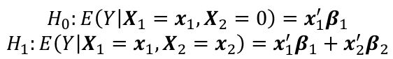
The null hypothesis is obtained by setting beta_2 = 0

The reasoning is that if RSS_𝜔 - RSS_Ω is small, the fit of the smaller model is almost as good as the larger model. On the other hand, if the difference is large the superior fit of the larger model would be perferred.

This suggests  (RSS_𝜔 - RSS_Ω)/RSS_Ω would be a potentially good test statistic where the denominator is used for scaling purpose

F Tests

Suppose the dimensions of Ω is p and that of 𝜔 is q. The general formula for the test is:

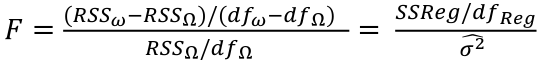
where df_Ω = n - p, and df_𝜔 = n - q

Thus, we would reject the null hypothesis if F > F^α _{p - q, n - p}

Simple Regression

Recall the ANOVA table for a simple regression:

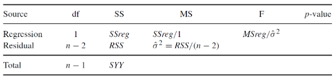
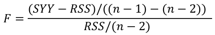
Under the null hypothesis:

The df is the number of n observations minus the number of estimated parameters: (n-1)

Under the alternative hypothesis:

Test of All the Predictors

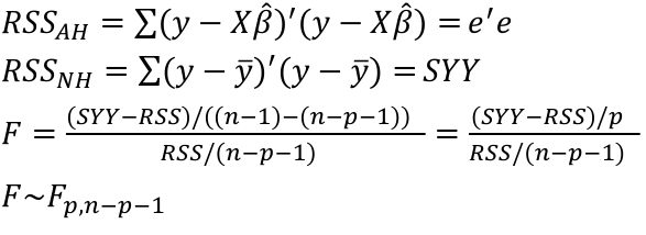
Where p is the number of regressors and n is the sample size.

One Predictor

Can a particular predictor be dropped from the model?

A t test can be used with (n - p - 1) degrees of freedom

The F test may be used as introduced earlier with a df of 1, n-p-1. t_i² here is exactly the F-statistic.

Dummy Variables and Analysis of Covariance

So far we have mostly seen quantitative variables in regression models, but many variables of interest are qualitative (sex, status, etc). To add such information to a model, we can set up a indicator/dummy variable.

For example, we could set up a variable X_i2 representing sex as 0 for type A and 1 for other for the i^th individual. The resulting model would look something like:

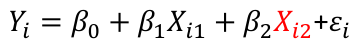
Where X_i2 is 0 when the individual is type A. So for type A:

But for any other type:

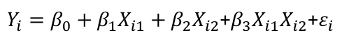
Models with Interaction

If we have a first-order regression model with an interaction we can represent it with an interaction term:

We can illustrate interaction as follows:

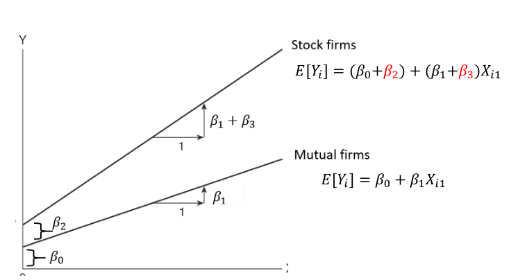
Beta2 indicates how much greater (smaller) the Y intercept for the class coded 1 than that of the class coded 0
Beta3 indicates how much greater (smaller) the slope for the class coded 1 then that of the class coded 0

Raw Mean

A raw mean is simply an average of the observations without considering other covariates. Least square means (sometimes called adjusted mean) are adjusted for other covariates, since it is estimated from a linear regression.

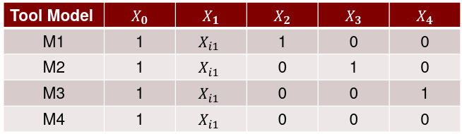
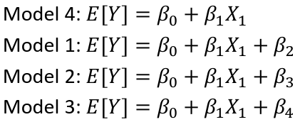
Qualitative Variable with 2+ Classes

If there are more than 2 classes to a qualitative variable, we require additional indicator variables in the regression model.

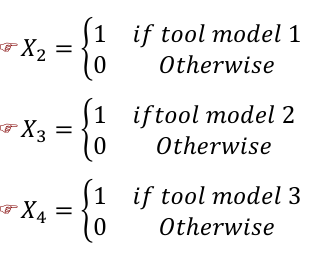
Resulting in a model like:

And the X matrix would look like:

Broken Stick Regression, Polynomial Regression, Splines

Transformations of the response and predictors can improve the fit and correct violations of model assumptions such as non-constant error variance. This chapter focuses on the transformation of predictors.

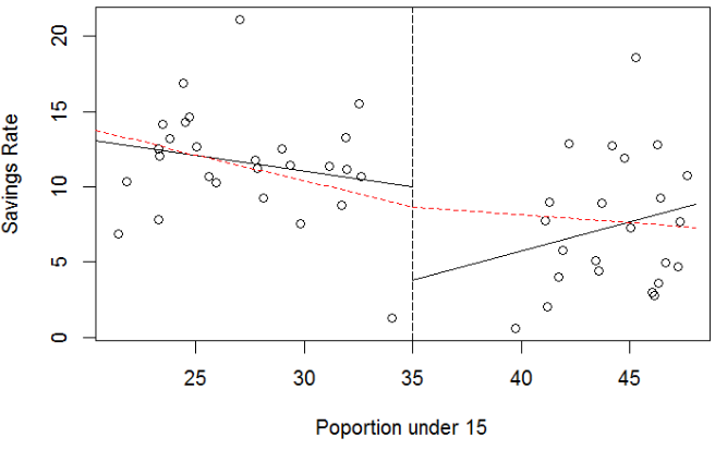
The idea behind Broken Stick Regression/Segmented Regression is that different linear regression models may apply in different regions of the data. We define two basis functions:

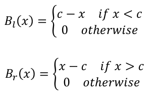
where c marks the division between groups. Bl(x) and Br(x) form a first-order spline basis with knot point c. Sometimes Bl(x) and Br(x) are called hockey-stick functions.

Polynomial Regression

Polynomial Regression models are frequently used curvilinear response models in practice. They make it easy to handle special cases of the linear regression model, however in reality this is not an exact representation.

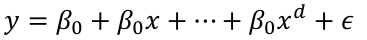
We choose d by adding terms until the added term is not statistically significant. Start with a large d and eliminate non-statistically significant terms starting with the highest order term.

Regression Splines

• Polynomials regression has:
  • the advantage of smoothness
  • the disadvantage that each data point affects the fit globally
• Broken stick regression method
  • Localized the influence of each data point to its particular segment
  • Do not have the same smoothness as with polynomials
• Use B-spline basis functions
  • Have both smoothness and local influence
  • Can overfit the model

 

Regression Diagnostics

The estimation and inference from the regression model depends on several assumptions. These assumptions need to be checked using regression diagnostics.

We divide the potential problems into three categories:

• Error: 𝜀 ~ N(0, 𝜎²I); i.e. the errors are:
  • Independent
  • Have equal variance
  • Are normally distributed
• Model: The structure part of model E[y] = Xβ is correct
• Unusual observations: Sometimes just a few observations do not fit the model but might change the choice and fit of the model

Diagnostic Techniques

• Graphical
  • More flexible but harder to definitively interpret
• Numerical
  • Narrower in scope but require no intution

Model building is often an interactive and interactive process. It is quite common to repeat the diagnostics on a succession of models.

Unobservable Random Errors

Recall a basic multiple linear regression model is given by:
    E[Y|X] = Xβ   and   Var(Y|X) = 𝜎²I

The vectors of errors is 𝜀 = Y - E(Y|X) = Y - Xβ; where  𝜀  is unobservable random variables with:
    E(𝜀 | X) = 0
    Var(𝜀 | X) =  𝜎²I

We estimate beta with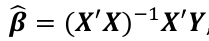

and the fitted values Y_hat corresponding to the observed value Y are: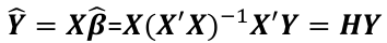
Where H is the hat matrix. Defined as: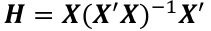

The Residuals

The vector of residuals e_hat, which can be graphed, is defined as:
    E(e_hat | X) = 0
    Var(e_hat | X) = 𝜎²(I - H)
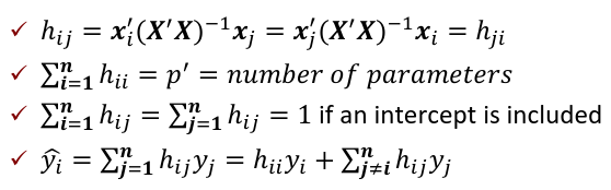
    Var(e_hat_i | X) = 𝜎²(I - h_ii); where h_ii is the i^th diagonal element of H.

Diagnostic procedures are based on the residuals which we would like to assume behave as the unobservable errors would.

Cases with large values of h_ii will have small values for Var(e_hat_i | X)

The Hat Matrix

The hat matrix H is n x n symmetric matrix

• HX = X
• (I - H)X = 0
• HH = H² = H
• Cov(Y_hat, e_hat | X) = Cov(HY, (I - H)Y| X) =  𝜎²H(I - H) = 0

h_ii is also called the leverage of the i^th case. As h_ii approaches 1, y_hat_i gets close to y_i.

Error Assumptions

We wish to check the independence, constant variance, and normality of the errors  𝜀. The errors are not observable, but we can examine the residuals e_hat.

They are NOT interchangeable with the error.

The errors may have equal variance and be uncorrelated while the residuals do not. The impact of this is usually small and diagnostics are often applied to the residuals in order to check the assumptions on the error.

Constant Variance

Check whether the variance in the residuals is related to some other quantity Y_hat and Xi

• e_hat against Y_hat: If all is well there should be constant variance in the vertical direction (e_hat) and the scatter should be symmetric vertically about 0 (linearity)
• e_hat against Xi (for predictors that are both in and out of the model): Look for the same things except in the case of plots against predictors not in the model, look for any relationship that might indicate that this predictor should be included.
• Although the interpretation of the plot may be ambiguous, one can be at least sure that nothing is seriously wrong with the assumptions.

Normality Assumptions

The tests and confidence intervals we used are based on the assumption of normal errors. The residuals can be assessed for normality using a QQ plot. This compares residuals to "ideal" normal observations.

Suppose we have a sample of n: x1, x2... xn. and wish to examine whether the x's are a sample from normal  distribution:

• Order the x's to get x(1) <= x(2).... <= x(n)
• Consider a standard normal sample of size n. Let z(1) <= z(2).... <= z(n)
• If x's are normal then E[x(i)] = mean + sd*z(i); so the regression of x(i) on z(i) will be a straight line

Many statistics have been proposed for testing a sample for normality. One of these that works well is the Shapiro and Wilk W statistic, which is the square of the correlation between the observed order statistics and the expected order statistics.

• H0 is that the residuals are normal
• Only recommend this in conjunction with a QQ plot
• For a small sample size, formal tests lack power
• For a large dataset, even mild deviations from non-normality may be detected. But there would be little reason to abandon least squares because the effects of non-normality are mitigated by large sample sizes.

Testing for Curvature

One helpful test looks for curvature in the plot. Suppose we have residual e_hat vs a quantity U where U could be a regressor or a combination of regressors.

A simple test for curvature is:

• To refit the model with an additional regressor for U^2 added
• The test is based on test testing the coefficient for U^2 to be 0
• If U does not depend on estimated coefficients, then a usual t-test of this hypothesis can be used
• If U is equal to the fitted values (which depends on the estimated coefficients) then the test statistic is approximately the standard normal distribution

Unusual Observations

Some observations do not fit the model well, called outliers. Some observations change the fit of the model in a substantive manner, called influential observations. If an observation has the potential to influence the fit, it is called a leverage point.

h_ii is called leverage and is useful diagnostics.

Var(e_hat_i | X) = 𝜎²(1 - h_ii)
    A large leverage will make Var(e_hat_i | X) small
    The fit will be forced close to y_i

= number of parameters
    An average value for h_ii is p'/n
    A "rule of thumb": leverage > 2p'/n should be looked at more closely

h_ij = x_i'(X'X)^-1x_j
    Leverage only depends on X, not Y

Suppose that the i-th case is suspected to be an outlier:

• We exclude point i-th case is suspected to be an outlier
• Recompute the estimates to get estimated coefficents and variance
• If y_hat_i - y_i is large, then case i is an outlier. To judge the size of potential outlier, we need to an appropriate scale:
  

  
  The variance is estimated by replaced variance with estimated variance. at i

• Assuming normal errors, the hypothesis E[y_hat_i - y_i] = 0 is given by
  

  

Alternative Method

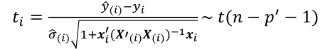
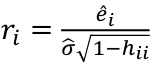
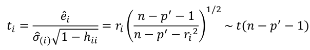
• Define standardized residual (internal studentized residual) as
  

  
  

• Then studentized residual (external studentized, jackknife, or cross-validated residual, Rstudent) can be calculated as:
  

  

Bonferroni Correction

Even though we might explicitly test only one or two large t_i by identifying them as large, we are implicity testing all cases. So, multiple testing correction such as Bonferroni correction should be implemented. Suppose we want a level alpha test:

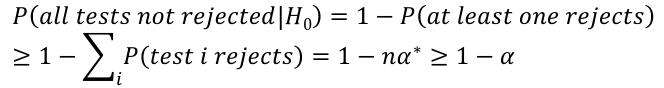
So it suggests that if an overall level alpha test is required, then a level should be alpha/n in each of the tests.

Notes on Outliers:

• An outlier in one model may not be an outlier in another when the variables have been changed or transformed
• The error distribution may not be normal and so larger residuals may be expected
• Individual outliers are usually much less of a problem in larger datasets. A single point will not have the leverage to affect the fit very much. It is still worth identifying outliers if these types of observations are worth knowing in the context.
• For large datasets, we only need to worry about clusters of outliers. Such clusters are less likely to occur by chance and more likely too represent actual structure.

When handling outliers:

• Check for a data-entry error first
• Examine the physical context, ex. the outliers in the analysis of credit card transactions may indicate fraud
• Exclude the point from the analysis but try re-including it later if the model is changed.
• Always report the existence of outliers even if they are not included in the final model!

Influential Observations

An influential point is one whose removal from the dataset causes a large change in fit. An influentual point may or may not be an outier or a leverage point.

Two meausures for identifying the infuential observations:

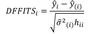
• Difference in Fits (DFFITS)
  

  

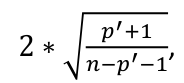
  An observation is influential if the absolute value is greater than:
  

  , where p is the number of parameters (predictors + 1)
  

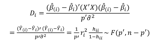
• Cook's Distance
  

  
  where p is the number of parameters (predictors + 1)
  

  • Di summarized how much alll of the fitted values change with the i-th observation is deleted
  • A "rule of thumb" is Cook Distance > 4/n should be looked at more closely
  • Di = 1 will potentially have important change in estimate
    • Di > .5 may be influential
    • Di >= 1 quite likely to be influential
    • If Di sticks out from others it is almost certainly influential
• Potential Outlier's percentile value using the F-distribution ~ F(p', n-p')
  • If < 10 or 20 percentile, little apparent influence
  • If > 50 percentile, highly influential
  • If in between, ambiguous

These rules are guidelines only, not a hard rule.

Code

## Test for normallity
gs <- lm(sqrt(Species) ~ Area + Elevation + Scruz + Nearest + Adjacent, gala)
g <- lm(Species ~ Area + Elevation + Scruz + Nearest + Adjacent, gala)

par(mfrow=c(2,2))
plot(fitted(g), residuals(g), xlab="fitted", ylab="Residuals")

qqnorm(residuals(g), ylab="Residuals")
qqline(residuals(g))

hist(g$residuals)

## Testing for curvature
library(alr4)
m2 <- lm(fertility ~ log(ppgdp) + pctUrban, UN11)
residualPlots(m2)
summary(m2)$coeff

## Testing for Outliers
g <- lm(sr ~ pop15 + pop75 + dpi + ddpi, savings)
n <- nrow(savings)
pprime <- 5   # number of parameters
jack <- rstudent(g)   # studentized residual
jack[which.max(abs(jack))]  # maximum studentized residual

# threshold for lower tail
qt(0.05/(50*2), df = n-pprime-1 , lower.tail=TRUE) 

#### influential points
cook <- cooks.distance(g)
n <- nrow(savings)
pprime <- 5

check <- cook[cook > 4/n]  # rule of thumb
sort(check, decreasing=TRUE) [1:5]  # list first five max

cook[cook>0.5]    # check Di>0.5
cook[(pf(cook, pprime, n-pprime)>0.5)] # use F-dist

influenceIndexPlot(g)

Variable Selection

Variable selection is intended to select the "best subset" of predictors. Variable selection shouldn't be separated from the rest of the model; Outliers and influential points can change the model we select. Transformations of the variables can have an impact on the model selection. Some iteration and experimentation is often necessary to find some better model.

The aim of variable selection is to construct a model that predicts or explains the relationships in the data. Automatic variable selections are not guaranteed to be consistent with these goals, so use these methods as a guide only.

The "best" subset of predictors:

• Explains the data in the simplest way
• Doesn't waste degrees of freedom with unnecessary predictors, which add noise
• Can save time or money by not measuring redundant predictors
• Doesn't include collinearity caused by too many variables trying to do the same job

There are two types of variable selections we will cover today:

• Stepwise testing approach - compares successive models
• The criterion approach - finds the model that optimizes some measure of goodness of fit

Model Hierarchy

Some models have a natural hierarchy, ex polynomial regression models (x² is a higher order term than x). When selecting variables it is important to respect the hierarchy. Lower order terms should not be removed from the model before higher order terms in the same variable.

Consider the model: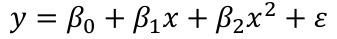

Suppose the summary shows that the term in x is not significant but x² is. If we removed x our model would become: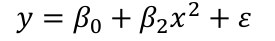

Then let's change the scale and change x to (x + a). Then the model would become:
The first order x reappears! The interpretation should not depend on the scale.

Scale changes should not make any important changes to the model.

Testing-Based Procedures

Backward Elimination

1. Start with all the predictors in the model
2. Remove the predictor with highest p-value greater than alpha
3. Refit the model
4. Remove the remaining least significant predictor provided its p-value is greater than alpha
5. Repeat 3 and 4 until all "non-significant" predictors are removed

Alpha is sometimes called the "p-to-remove" and does not have to be 5%. For prediction purpose, 15-20% cutoff may be best.

Forward Selection

Reverses the backwards method

1. Start with no variables
2. For predictors not in the model, check the p-value if they are added to the model. We choose the one with lowest p-value less than alpha
3. Continue until no new predictors can be added

Stepwise Regression

Combination of backwards elimination and forward selection.

• At each stage, a variable may be added or removed and there are several variations on how this is done.
• The stepwise regression can be done top-down (alternate drop step with add step) or bottom-up (alternate add step with drop step)

Notes on Testing-Based Procedures

• Possible to miss the "optimal" model due to "one-at-a-time" nature of adding/dropping variables
• The p-values used should not be treated too literally as there is so much multiple testing occurring
• The procedures are not directly linked to final objectives of prediction or explanation
• Variables that are dropped can still be correlated with the response. It is just that they provide no additional explanatory effect beyond those variables already included in the model
• Stepwise selection tends to pick models smaller than desirable for prediction purpose

Criterion-Based Procedures

Criteria for model selection are based on lack of fit of a model and its complexity.

Some possible criteria:

• Akaike Information Criterion (AIC):
  • -2 max log-likelihood + 2p'
  • n*log(RSS/n) + 2p'
• Bayes Information Criterion (BIC):
  • -2 max log-likelihood + p' log(n)
  • n*log(RSS/n) + log(n) * p'

Note p' is the number of parameters including the intercept.

Small values of AIC and BIC are preferred. So better candidate sets will have smaller RSS and a smaller number of terms p. Larger models fit better and have smaller RSS but use more parameters. The goal is to find a balance between RSS and p.

BIC penalizes larger models more heavily. Smaller models are perferred in BIC as compared to AIC.

Adjusted R²

R² = 1 - RSS/SSY

• Adding variables can only decrease RSS and increase R²
• Not a good criterion as it always perfers the largest model
• Important to pay attention for significant changes of RSS!

Another commonly used criterion is adjusted R², written R_a²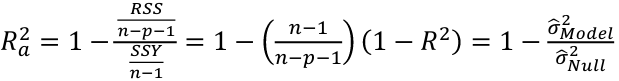

Mallow's C_p Statistics

A good model should predict well, so the average mean square error of prediction might be a good criterion: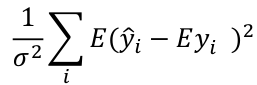
which can be estimated by the C_p statistic: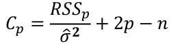

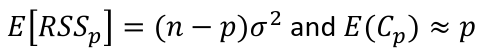
where sigma squared is from the model with ALL predictors and RSS_p indicates that RSS from a model with p parameters.

• For the full model C_p = p
• If a p-predictor model fits then:
  

  

• If a model has a bad fit, C_p will be much larger than p
• We desire models with small p and C_p around or less than p

R Code

install.packages("faraway")
library(faraway)
data(state)
names(state)
statedata <- data.frame(state.x77, row.names=state.abb)

names(statedata)
write.csv(statedata, file="statedata.csv", quote=FALSE, row.names=F)

############# from here
## the data were collected from U.S. Bureau of the Census. 
## use life expectancy as the response
## the remaining variables as predictors

statedata <- read.csv("statedata.csv")
g <- lm(Life.Exp ~ ., data = statedata)
summary(g)

### backward elimination
g <- lm(Life.Exp ~ ., data = statedata)
summary(g)$coefficients

g <- update(g, .~ . - Area)
summary(g)$coefficients

g <- update(g, .~ . - Illiteracy)
summary(g)$coefficients

g <- update(g, .~ . - Income)
summary(g)$coefficients

g <- update(g, .~ . - Population)
summary(g)$coefficients
summary(g)

## step(lm(Life.Exp ~ ., data = statedata), 
#	scope=list(lower=as.formula(.~Illiteracy)), direction="backward")

### the variables omitted from the model may still be related to the response
summary(lm(Life.Exp ~ Illiteracy+Murder+Frost, statedata))$coeff
 
## forward
f <- ~Population + Income + Illiteracy + Murder + HS.Grad + Frost + Area
m0 <- lm(Life.Exp ~ 1, data = statedata)
m.forward <- step(m0, scope = f, direction ="forward", k=2)

## hand calculate the AIC value
aov(lm(Life.Exp ~ Murder, data=statedata))
# AIC = n*log(RSS/n) + 2p

n <- nrow(statedata)
n*log(34.46/n)+2*2

extractAIC(m.forward, k=2)		# by default k=2, AIC
extractAIC(m.forward,k=log(50))		# k=log(n), BIC

## final model using AIC
summary(m.forward)$coefficients

## use BIC
n <- nrow(statedata)
m.forward.BIC <- step(m0, scope = f, direction ="forward", 
			k=log(n), trace=FALSE)
summary(m.forward.BIC)$coefficients


### backward
m1 <- update(m0, f)
m.backward <- step(m1, scope = c(lower= ~ 1), 
			direction = "backward", trace=FALSE)
summary(m.backward)$coefficients

### stepwise
m.stepup <- step(m0, scope=f, direction="both", trace=FALSE)
summary(m.stepup)$coefficients

########## about Cp
install.packages("leaps")
library(leaps)
leaps <- regsubsets(Life.Exp ~ ., data = statedata)
rs <- summary(leaps)
par(mfrow=c(1,2))
plot(2:8, rs$cp, xlab="No. of parameters",
		ylab="Cp Statistic")
abline(0,1)

plot(2:8, rs$adjr2, xlab="No. of parameters",
		ylab="Adjusted R-Squared")
abline(0,1)
names(rs)

rs

Midterm Cheat Sheet

Linear Regression Predicting a CI new obs adds a 1 to se(y): 𝛽0 + 𝛽2x +/- t*	Multiple Linear Regression and Estimation 𝐻0 : 𝛽1 = 𝛽2 = 𝛽3 = ⋯ = 𝛽𝑝 = 0   v.s.  𝐻1 : not all 𝛽𝑘 = 0, 𝑘 = 1, … , 𝑝 rejection rule of 𝑡 >= t(1 − alpha/2; 𝑛 − 𝑝 − 1)
Model Fitting: Inference dfΩ = n - p, and df𝜔 = n – q Reject the null hypothesis if F > Fα p - q, n – p	Dummy Variables and Analysis of Covariance Consider a Xi2 for which is 0 for – and 1 for +: An interaction between Xi1 and Xi2: A model with multiple categorical variables:
Regression Diagnostics Assumptions:     • Error:  ~ N(0, SD2I);          ◦ Independent         ◦ Equal Variance         ◦ Normally Distributed     • Model: E[y] = Xβ is correct     • Unusual observations        Leverage Points: data point with unusual x-value       The Hat Matrix – n*n matrix hii is the leverage of the ith case leverage > 2p’/n should be looked at closely Outliers: Unusual observation on x or y axis Calculate the t-test and compare abs with limit: abs(qt(.05/(n*2), df = n - pprime - 1, lower.tail = T))	Influential Points: causes changes to regression     Difference in Fits: with a threshold of Where p’ is the number of parameters      Cook's Distance: with a threshold of Di > 4/n should be looked at Di > .5 possible influence Di >= 1 very influential Error: a plot of e_hat should     • have constant variance     • have no clear pattern     • H0: residuals are normal Shapiro-Wilk normality test H0: Residuals are normally distributed Bonferroni Correction: Divide alpha by n
Variable Selection Backwards Elimination: Start model with all the predictors Remove the predictor with highest p-value greater than alpha Refit the model Remove the remaining least significant predictor provided its p-value is greater than alpha Repeat 3 and 4 until all "non-significant" predictors are removed Cutoff p significance can be 15-20% for testing Forward Selection: Start model with no predictors For predictors not in the model, check the p-value if they are added to the model. We choose the one with lowest p-value less than alpha Continue until no new predictors can be added Stepwise regression: A combination of the two	Selection Criteria: Akaike Information Criterion (AIC):      • -2 max log-likelihood + 2p'      • n*log(RSS/n) + 2p' Bayes Information Criterion (BIC):      • -2 max log-likelihood + p' log(n)      • n*log(RSS/n) + log(n) * p'  Adjusted R2: R2 = 1 – RSS/SSY Mallow’s Cp Statistic: Avg MSE of prediction If a p-predictor fits then: We desire models with small p and Cp around or less than p

R Code Snippets

# Model with only beta_0 sr_lm0 <- lm(y ~ 1, data=sr) # Full model sr_lm1 <- lm(y ~ ., data=sr) sr_syy <- sum((savings$sr - mean(savings$sr))^2) sr_rss <- deviance(sr_lm1) # F = ((SYY -RSS)/((n-1) - (n-2))) / (RSS / (n - 1)) sr_num <- (sr_syy - sr_rss)/(df.residual(sr_lm0) - df.residual(sr_lm1)) sr_den <- sr_rss / df.residual(sr_lm1) sr_f <- sr_num / sr_den # dfΩ = n - p, and df𝜔 = n - q pf(sr_f, df.residual(sr_lm0) - df.residual(sr_lm1), df.residual(sr_lm1), lower.tail = F) # β=(XI X)−1 XIY beta <- solve(t(x)%*%x)%*%(t(x)%*%y) # Pearson's cor(lin_reg$fitted.values, lin_reg$residuals, method="pearson") # Stratify variables by a factor by(depress, depress$publicassist, summary) # Welsh's Two Sample T-test # For difference in means t.test(assist$cesd, noassist$cesd) # or t.test(data.y ~ factor) # CI of LS means based on covariates library(lsmeans) lsmeans(reg, ~Type) # Apply a mean function to an array # split on a factor tapply(assist$cesd, assist$assist, mean) # When a regression factor has # more than two categories reg <- lm(Pulse1 ~ Height + Sex + Smokes + as.factor(Exercise))

# Cook's Distance cook <- cooks.distance(reg) cook[cook > 4/n] # Shapiro Test for normallity shapiro.test(reg$residuals) # Studentized residuals stud <- rstudent(reg) # Threshold for lower tail of # studentized resids with correction lim = abs(qt(.05/(n*2), df = n - pprime - 1, lower.tail = T)) stud[which(abs(stud) > lim)] # Hat values hat <- hatvalues(reg) lev <- 2 * pprime / n hat[hat > lev] # Forward selection forward <- ~ year + unemployed + femlab + marriage + birth + military m0 <- lm(divorce ~ 1, data = usa) reg.forward.AIC <- step(m0, scope = forward, direction = "forward", k = 2) n <- nrow(usa) # AIC = n*log(RSS/n) + 2p' n*log(162.1228/n)+2*6 extractAIC(reg.forward.AIC, k=2) # BIC reg.forward.BIC <- step(m0, scope = forward, direction = "forward", k = log(n)) extractAIC(reg.forward,k=log(n)) # BIC = n*log(RSS/n) + p'*log*n) n*log(162.1228/n)+6*log(n) library(leaps) leaps <- regsubsets(divorce ~ .) rs <- summary(leaps) par(mfrow=c(1,2)) plot(2:7, rs$cp, xlab="No. of parameters", ylab="Cp Statistic") abline(0,1)

Tree Based Methods

Classification and regression trees can be generated from multivariable data sets using recursive partitioning with:

• Gini index or entropy for a categorical outcome
• Residual sum of squares for a continuous outcome

We can use cross-validation to assess the predictive accuracy of tree-based models.

Non-Linear Regression

Polynomial Regression adds extra predictors by raising original predictors to a power. Provides a simple way to provide a nonlinear fit to data.

Step functions/Broken stick regression cuts the range of a variable into K distinct regions. Fits a piecewise constant function/regression line.

Regression splines and smoothing lines is an extension of the two above. The range of X is divided into K distinct regions. Within each region a polynomial function is fit to the data. It is constrained in a way which smoothly joins at the region boundaries, or knots. It can produce an extremely flexible fit if there are enough divisions.

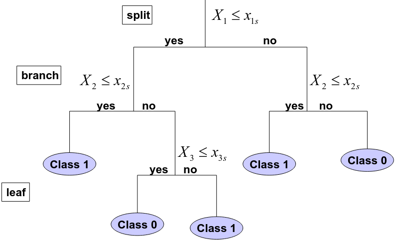
Classification and Regression Trees

Classification and Regression Trees (CART) are a computer intensive alternative to fitting classical regression models. CART works very well for highly non-linear problems.

• These involve stratifying or segmenting the predictor space into a number of simple regions.
• In order to make a prediction for a given observation we typically use the mean or mode of the training observations in the region which it belongs to.
• Classification trees apply when the response it categorical
• Regression trees apply when the response is continuous

A regression tree is basically just a multiple linear regression model with indicator variables that represent the branches of the tree.

Regression Tree

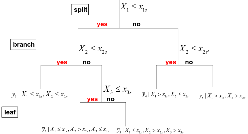
Note: Number of leaves = complexity

1. We divide the predictor space into J distinct and non-overlapping regions R₁, R₂, R_j.
2. The fitted value in a region R_j is simply the mean of the response values in this region :
   

   

Goal: The regions are identified to minimize:

Where Rj is the rectangle corresponding to the jth terminal node and y_bar_j is the mean of the training observations in R_j

A complete search is not feasible and we take a top-down, greedy approach known as recursive binary splitting.
Top-down: Start from the top of the tree
Greedy: Best solution at each node of the tree (local rather than global)

Recursive Binary Splitting

Input: "explanatory" variables and outcome Y

For each variable X_g,
without splitting X_g, the variable Y has a certain variability

Splitting the data by X_g < s, then the new RSS is:

• Identify the split of the variable to minimize the new RSS
• Identify the variable whose split minimizes the new RSS
• Repeat in each region in a recursive way

Residual Mean Deviance

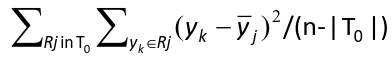
T₀ = tree; | T₀ | = number of leaves; y_bar = mean in region R_j

Pruning

Build a large tree and fold terminal branches back. This can be based on a maximum number of leaves, or use cost-complexity pruning.

Typically pruning overfits the data (too many splits). A smaller tree with fewer splits might lead to better interpretation at the cost of higher residual deviance.

Possible alternatives: Build the tree only so long as the decrease in the RSS due to each split exceeds some threshold. This strategy may terminate too early.
The idea here is to minimize RSS
For a given alpha search for the tree T nesting into T₀ that minimizes: where alpha=cost; |T| number of leaves
Use a heuristic search to find alpha

Cart for Prediction

To access the accuracy of a regression tree to predict Y in new patients, you can evaluate the predictive accuracy by using a training and testing set.

Classification Tree

Input: Explanatory variables and a class label for different samples

The objective is to choose the tree which maximizes the classification accuracy

The procedure (same as regression tree with 2 differences):

• The fitted value at each terminal node is the most frequent label
• The deviance is replaced by a "measure of information" or classification error

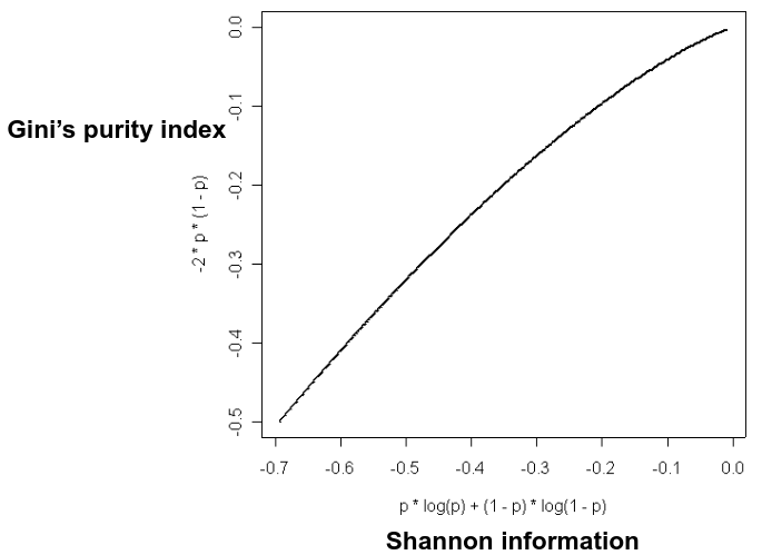
Shannon Entropy

Shannon entropy is the most common measure of (Lack of) information content of a binary variable: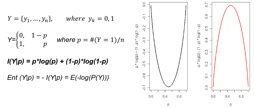

Gini's Impurity Index

Gini's Impurity Index is the information content of a binary variable.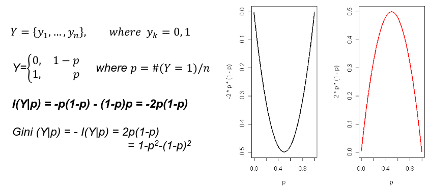

Best Split

For each variable:

• Compute the information gain for each x_gs
• Identify the split that gives the largest information gain

Do this linear search for each variable and identify the optimal split and maximum gain of information.

Split the node by using the variable that gives the largest information gain with a binary split.

Typically Gini index is used for growing a tree, and misclassification error is a good metric for pruning a tree.

Pros and Cons of Trees

• Very easy to explain, even more so than linear regression
• Some people think decision trees more closely mirror human decision-making than previously seen classification and regression.
• Trees can be displayed graphically and are easily interpreted by a non-expert
• Trees can easily handle qualitative predictors without the need to create dummy variables.
• HOWEVER, trees are not precise for prediction. By using methods like bagging, random forests, and boosting the predictive performance can be substantially improved.

Bagging, Boosting, and Random Forest

• Bagging is a useful procedure when the goal of analysis is prediction
  • Generate many subsets of data by randomly sampling subsets of the data (with replacement so the subject can appear more than once in the same set)
  • In each subset generate a tree without pruning
  • Using the average of the prediction from all the trees to compute the final prediciton
• Sampling with replacement to estimate statistical quanitities is known as bootstrap
• Random Forest is similar to bootstrap
  • The difference is in each bootstrap sample the set of covariates to build the tree is randomly selected selected rather than using all of them
• Boosting grows a family of trees sequentially

Bagging and Random Forest improve prediction at the cost of interpretability.

One can generate an importance value of each covariate as the average improvement of RSS (or entropy or Gini index) due to the covariate in each tree and rank the covariates by this importance value.

The larger the average change in deviance, the more important the variable.

Classification Rules

The data is split into testing and training sets. We use the training set to build the classification rule; and the test set to evaluate how the classification rule labels new cases with known label.

Accuracy is the rate of correctly classified labels in the test set.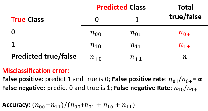

Sensitivity is a metric of true positive detection and shows whether the rule is sensitive to identify positive outcomes:

Specificity is the measure of true negative detection and showos whether the rule is specific in detection of negative outcomes:

Principal Component Analysis

The goal of supervised learning methods (regression and classification) is to predict outcome/response variable Y using a set of p features (X1, X2... Xp) measured on n observations. We train the machine on 'labeled' data to predict outcomes for unforeseen data.

Unsupervised learning is a set of tools (principle component analysis and clustering) intended to explore only a set of features (X1, X2... Xp) and to discover interesting things about these features. This is often performed as part of an exploratory data analysis.

The challenge of unsupervised learning is that is is more subjective than supervised learning, as there is no simple goal for the analysis such as prediction of a response.

Principle Component Analysis (PCA)

Visualize n observations with measurements on a set of p features as part of an exploratory data analysis. Do this by examining 2-dimensional scatterplots. PCA produces a low-dimensional representation of a dataset that contains as much variation as possible.

Input of PCA is a data matrix in which the columns are centered to have mean 0. Typically the columns represent variables (age, weight, etc) and rows represent different subjects.

Output of PCA is a data matrix Y in which the columns are linear transformations of the columns of X, and they are uncorrelated.

In general the columns has n rows and p columns (variables).

Method

PCA uses orthogonal transformation to convert the columns of X into new variables called principal components that are:

• Linear combinations of the original variables
• Uncorrelated
• Sorted so that the first PC has the largest variance and the rest are descending
• We can have at most as many PCs as columns, assuming p < n

The first principal component is the normalized linear combination of the vectors x1, ..., xp that has the largest variance. By normalized we mean: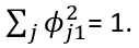

Where the theta elements of the above are loadings of the first principal component. We constrain the loadings so that their sum of squares is equal to one, since otherwise setting these elements to be arbitrarily large in absolute value could result in an arbitrarily large variance.

Calculating the First Principal Component

Assuming that the variables Xi are centered, we search for the loadings that maximize the sample variance of teh first PC, subject to the constraint above that sum of theta_j1^2 = 1.

We refer y11, y21, ..., yn1 as the scores or realized values of the first principal component where:

The average of yi1 (the scores of the first PC) is 0 since it is centered. The sample variance of the values of the n values of yi1 is: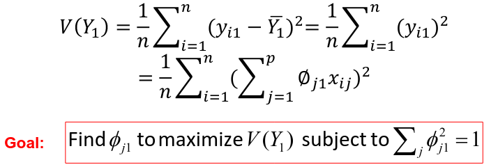

The loading vector theta_1 with elements theta_11, theta_21, ..., theta_p1 defines a direction in feature space along which the data vary the most.

If we project the n data points x1, x2, ..., xn onto this direction, the projected values are the principal component scores y11, y21, ..., yn1 themselves.

Calculation of the Second Principal Component

After we find 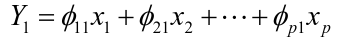 we can calculate the second PC:

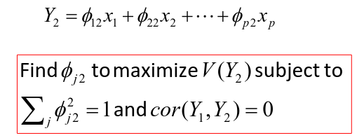
And so on until all PCs are found. These calculations can be done using the "singular value decomposition".

In R the 'prcomp()' function computes principal components by using a singular value decomposition.

The advantage of using PCA is that we hope to end up with a number of components that is smaller than the number of variables p.

We can use PCA for data reduction techniques. If 2 or 3 PCs explain a large portion of the total variance, then we can use these 2 or 3 variables for analysis rather than the whole set.

Spectral Decomposition

The spectral decomposition recasts a matrixx in terms of it eignenvalues and eigenvectors. The representation turns out to be very useful.

Let M be a real symmetric d x d matrix with eigen values lambda_1, lambda_2, ..., lambda_d and corresoinding orthonormal eigenvectors u1, u2, ..., ud then:

R Code

### Example 1
head(USArrests)
dim(USArrests)
sqrt(apply(USArrests,2,var))

plot(USArrests)
# compute principal components
pca1 <- prcomp(USArrests, scale=T)
pca1
(13.2 -mean(USArrests$Murder))/sqrt(var(USArrests$Murder))*( -0.5358995) +
  (236-mean(USArrests$Assault))/sqrt(var(USArrests$Assault))*(-0.5831836) +
  (58-mean(USArrests$UrbanPop))/sqrt(var(USArrests$UrbanPop))*(-0.2781909) +
  (21.2-mean(USArrests$Rape))/sqrt(var(USArrests$Rape))*(-0.5434321)

sum(((USArrests[1,]-pca1$center)/pca1$scale)*pca1$rotation[,1])

## generate summary of loadings
summary(pca1)
plot(pca1)

# extract principal components
pca1$x[1:5,]

# plot PCs
plot(pca1$x[,1:2])
biplot(pca1)

Intro to Cluster Analysis

Clutsering refers to a very broad set of techniques for finding subgroups, or clusters, in a data set. When we cluster the observations, we partition the profiles into distinct groups so that the profiles are similar within the groups but different from other groups. To do this, we must define what makes observations similar or different.

PCA vs Clustering

Both clustering and PCA seek to simplify the data via a small number of summaries, but their mechanisms are different:

• PCA searches for a low-dimensional representation of the observations that explains a good fraction of the variance
• Clustering looks to find homogeneous subgroup among the observations

Notation

Input is data with p variables and n subjects

A distance between two vectors i and j must obey several rules:

• The distance must be positive definite, d_ij >= 0
• The distance must be symmetric, d_ij = d_ij, so that the distance from j to i is the same as the distance from i to j
• An object is zero distance from itself, d_ii  = 0
• The triangle rule - When considering three objects i, j and k the distance from i to k is always less than or equal to the sum of the distance from i to j and the distance from j to k
  d_ik <= d_ij + d_jk

Clustering Procedures

• Hierarchical clustering: Iteratively merges profiles into clusters using a simple search. Start with each profile/cluster and end with one 1. The clustering procedure is represented by a dendrogram.
• K-mean clustering: Start with a per-specified number of clusters and random allocation of profiles to clusters. Iteratively move profiles from one cluster to the other to optimize some criterion. End up with the same number of clusters.

K-Means Clustering

We partition the K clusters so that we maximize the similarity within clusters and minimize the similarity between clusters.

We can represent the data with a vector of means, which is the overall profile or cluster: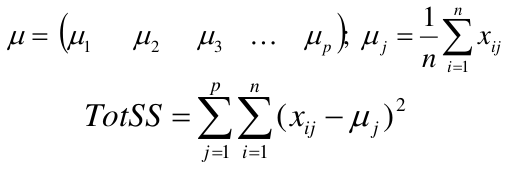

Supposed we split the data into 2 clusters, C1 with 𝑛1 observations of the p variables, and C2 with 𝑛2 observations of the p variables. We would have two different vectors of means representing the centroids of the clusters. The total sum of squares within clusters would be:

And we seek to keep WSS small, but it is NOT guaranteed to give the minimum WSS so ideally one should start from different initial values.

• Start with K "random" clusters by assigning each of the n profiles to one of the K clusters at random
• Iterate until no more changes are possible:
  • For each of the K clusters, compute the cluster profile (centroid)
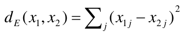
  • Assign each observation to the cluster whose centroid is closest (using Euclidean distance)
    

    

Example with K = 3, p = 2: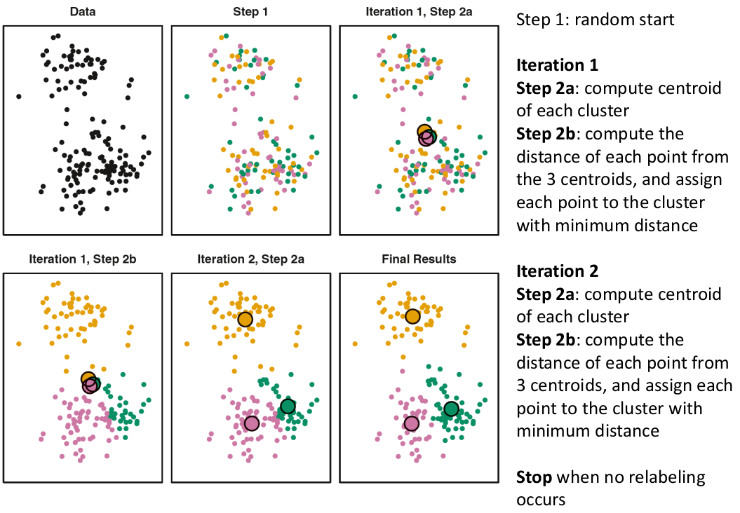

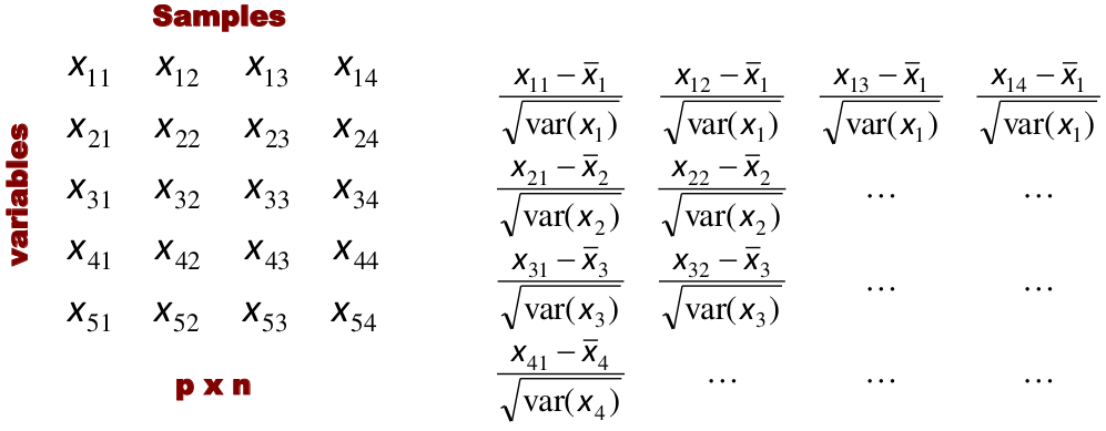
Standardization

When the variables are measured on different scales the measurement units may bias the cluster analysis. The Euclidean distance is not scale invariant.

Hierarchical Clustering

This is an alternative approach that does not require a fixed number of clusters. The algorithm essentially rearranges profiles so that similar profiles are displayed next to each other in a tree (dendrogram) and the dissimilar profiles are displayed in different branches.

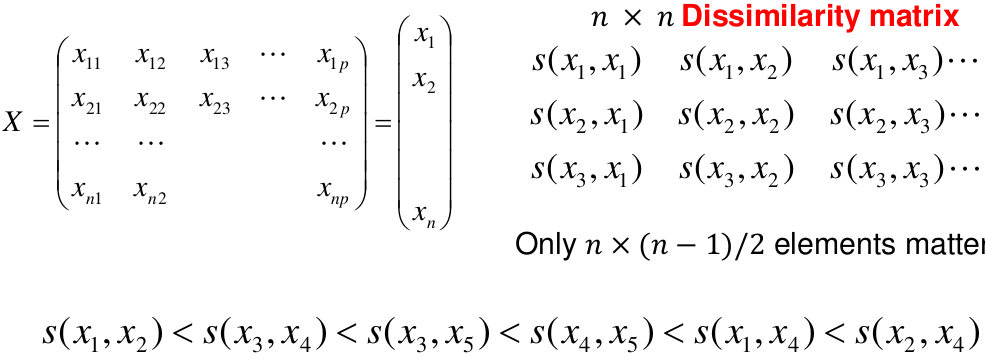
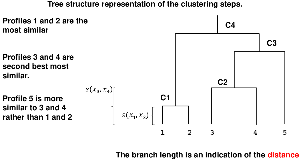
We do this we define the similarity (distance) between:

• Two profiles: s(xi, xi)
• A profile and a cluster: s(xc, xi)
• Two clusters: s(xc, xc)

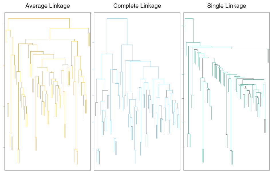
Similarity Between Clusters

Complete-Linkage Clustering

• Also known as the maximum or furthest-neighbor method
• The distance between two clusters is calculated as the greatest distance between members of the relevant clusters
• This method tends to produce very compact clusters of elements and the clusters are often similar in size

Single-Linkage Clustering

• Referred to as the minimum or nearest neighbor method
• The distance between two clusters is calculated as the minimum distance between members of the relevant clusters
• This method tends to produce clusters that are 'loose' because clusters can be joined if any two members are close together. In particular, this method often results in 'chaining' or sequential addition of single samples to an existing cluster and produces trees with many long, single-addition branches.

Average-Linkage Clustering

• The distance between clusters is calculated using average values. There are various methods used for calculating this average. The most common is the unweighted pair-group method average (UPGMA), where each average is calculated from the distance between each point in a cluster and all other points in another cluster and the 2 clusters with the lowest average distance are joined together into a new cluster.

Centroid Clustering

• Related methods substitute the centroid for the average.

Complete and average linkage are similar, but complete linkage is faster because it does not require recalculation of the similarity matrix at each step.

Detection of Clusters

Inspection of the QQ-plot would inform about the existence of clusters in the data.

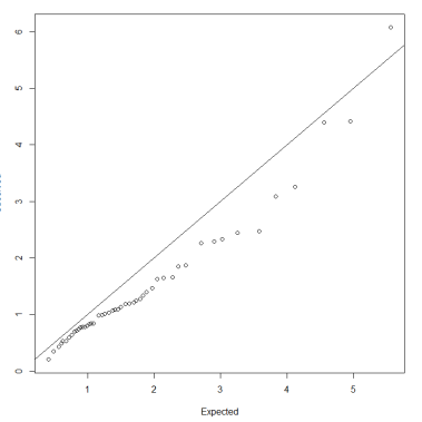
• Observed and “expected” distances are statistically indistinguishable would suggest that there are no clusters in the data
• Departure of the QQ-plot from the diagonal line would suggest that there are clusters

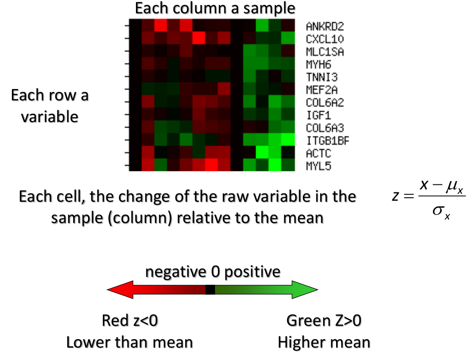
We can also use a 95%-tile to detect the number of clusters using extreme percentiles of the reference distribution. The idea is to color the entry of the data set, so that the colors represent the standardized difference of the cell intensity from a baseline. Typically, columns are samples and rows are variables.

 

Classification

Classification is often used to describe modeling of a categorical outcome.

In binary classification the outcome is two possible values/classes and the goal is the predict the correct class using covariates.

Classification rule: A mathematical function to predict the outcome of a new sample unit when the values of the covariates are known.

Common Classification Problems

• Molecular diagnostic: Using values of gene products (such as biomarkers) develops a diagnostic tool for early detection of diseases.
• Classification of cancer type: Different sub-types of cancer are characterized by a combination of specific markers that are on/off. Gene based classification rules can be used to increase the specificity of the diagnosis.
• Classification of drug response
• Risk prediction

Types of Classifiers

• Regression-based:
  • Logistic regression, CART
• Example-based:
  • KNN
• Based on Bayes theorem:
  • Discriminant analysis
• Ensemble of classifiers

To evaluate a classifier, split the data into a training and test set. Use the training set to build the classification rule and the test set to evaluate how the classification rule labels new cases with known label.

Logistic Regression

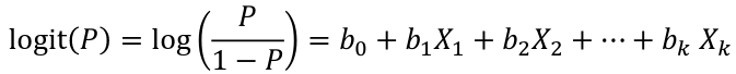
b_i, i = 0,1... k can be estimated using Maximum Likelihood

To estimate the probability of a binary outcome as a function of covariates with logistic regression: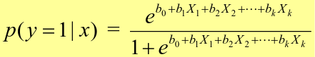

How to Pick Classification Rule

We can use the above formula for x in [0,1] to generate thresholds based on the predicted value to decide how to classify.

Accuracy is the rate of correctly classified labels in the test set: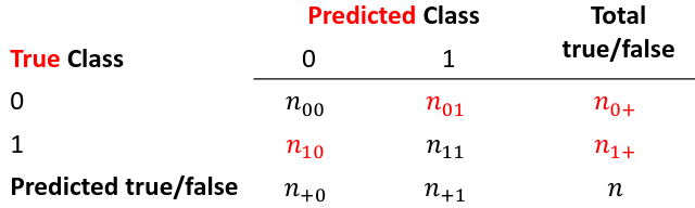

Misclassification error:
False positive: prediction 1 and true is 0; n01 / n0+
False negative: predict 0 and true is 1; Fn10 / n1+
Accuracy: (n00 + n11) / (n00 + n01 + n10 + n11)

Sensitivity (recall) the metric of true positive detection and shows whether the rule is sensitive to identify positive outcomes:  1 - n10 / n1+ = n11/n1+ = 1 - FNR

Specificity is the measure of true negative detection and shows whether the rule is specific in detection of negative outcomes:  1 - n01 / n0+  =  n00 / n0+ = 1 - FPR

You CANNOT maximize sensitivity and specificity simultaneously. Maximum sensitivity test always says 1, maximum sensitivity always says 0.

Positive/Negative predicted values: The number of correct all predicted positive/negative values

ROC (Receiver Operating Characteristics) Analysis

The ROC curve is a population graphic for simultaneously displaying the two types of errors for all possible thresholds.  They are useful for comparing different classifiers since they take into account all possible thresholds.

The overall performance of a classifier, summarized over all possible thresholds is given by the area under the ROC curve (AUC). An ideal ROC curve will hug the top-left corner, so the larger the AUC the better the classifier.

We expect a classifier that performs no better than chance to have an AUC of .5

Steps to Build and Evaluate Classification Rule:

1. Generate training and test set
2. Generate the classification rule using the training set;
3. Generate the predicted rules in the test set;
4. Use ROC analysis to decide the threshold that gives a good balance between sensitivity and specificity.
5. The next examples will show a variety of methods to generate classification rules (so step 2)

The previous chapter describes methods to create classification trees and K-nearest neighbor.

Discriminant Analysis

Logistic regression involves directly modeling P(Y = k | X = x) using logistic function. An alternative approach will model the distribution of the predictors X separately in each of the response classes, then use Bayes theorem to flip these around into estimates for P(Y = k | X =x)

Assuming the covariate x is normally distributed: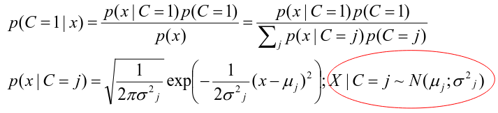

Binary outcome: Classify as 1 if p(C = 1 | x) > p(C = 0 | x)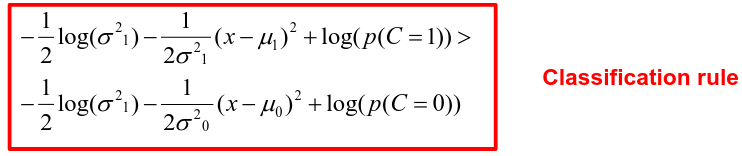

A special case when the variances of X in the groups are the same: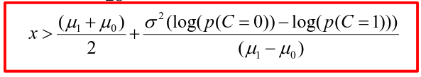

More than One Feature

To extend this approach to multiple covariates, one needs to decide:

1. How to model the correlation of the covariates within each group defined by the outcome
2. If the correlation of the covariates changes in different groups

LDA - assumes equal variance-covariance structure between groups
QDA - assumes group specific variance covariance matrices
LDA/QDA models all covariates as normal distributions

Summary

For each method:

1. Fit the classification model using training data
2. Evaluate the classification accuracy in test data using ROC analysis
3. Can also choose a “best” threshold to optimize sensitivity/specificity
4. Compare different classifiers by their AUC

The final classifier should be trained on all data to be used for future applications

There is no single "Best Classification Method". There is clear evidence that different methods work better in some data and worse in others. Thus, we often use the prediction probabilies of various classifiers to build an ensemble, using prediction probabilities from various rules. This is limited as there is no description of mechanism, useful only for prediction.

Two-Way ANOVA

We've learned about One-Way Analysis of Variance (ANOVA) previously, it is a regression model for one continuous outcome and one categorical variable. It allows us to compare the means of the groups to detect significant differences.

A one-way fixed-effects ANOVA is an extension of the two-sample t-test. There are factors, categorical variables, and levels, individual groups of the factor which represent different populations. Balanced design contain the same number of individuals in each level. This is a special case of linear regression. 

Assumptions of one-way ANOVA:

• The data are random samples from k independent populations
• Within each population the dependent variable is normally distributed
• The observations are independent
• The population variance of the dependent variable is equal in all groups (homoscedasticity)

H₀: The mean level is independent of the factor

Ex. The mean testosterone level is independent of smoking history. A conclusion might be "there is evidence that testosterone level is significantly different in at least two of the smoking history groups.

We test the hypothesis by decomposing the overall variance into "explained" and "residual" variances and comparing them.

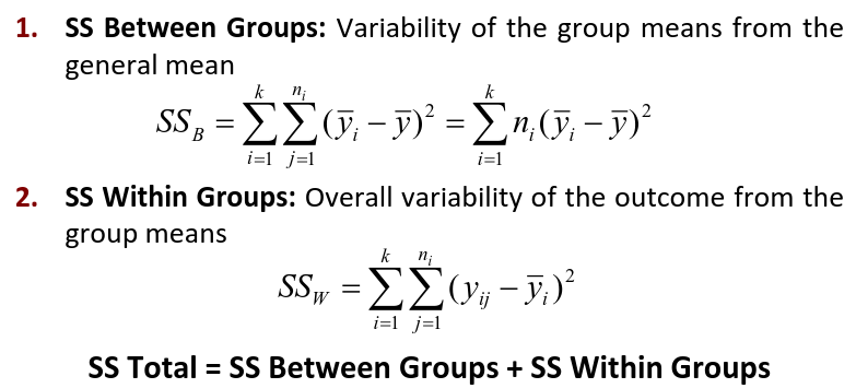
Where N is the total sample size and k is the number of groups
SSB represents the variability due to the treatment effect. SSW represents the residual variability.

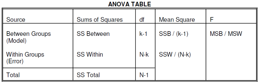
We compare the F statistic to the critical value of F with [(k - 1), (N - k)] degrees of freedom to test the null hypothesis of equal means.

Multiple Comparisons Procedures

To find which means are different from each other we should make all pairwise comparisons (k*(k-1)/2). This introduces the multiple tests issues and increases likeliness of type I and II errors. Multiple comparison procedures take into account the total number of comparisons being made by lowering the significance level for each test so that the overall significance level is still fixed at some level alpha.

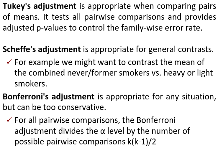
All  of these adjustments are appropriate when comparing pairs of means. Tukey's is the most powerful and provides exact p-values when the group sizes are equal. Scheffe's procedure is more powerful than Bonferroni's procedure, in general.

We can also write ANOVA as a linear regression model where the parameter alpha_i are the group effects (difference of effect between group i and group 1)

Two Way ANOVA

Two way ANOVA is a regression model for one continuous outcome and two categorical variables. We analyze two-way ANOVA experiments using additive and interaction models.

Critical assumptions:

• Observations at different factor levels are samples from normal distributions
• The variances of the different populations are the same

An experiment may also contain replication, for example consider the following tables: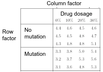

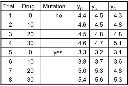
Both are the same data where the two factors are drug dosage and mutation, and we have 3 replications.

We can create summaries of the means: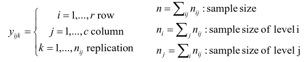

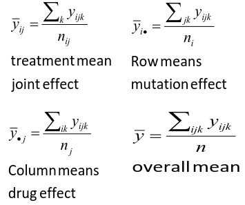
Possible Models

Interaction model: The effect of each factor changes as the other factor levels vary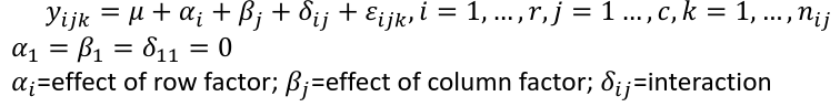

Additive model: The effect of each factor doesn't change as the other factor levels vary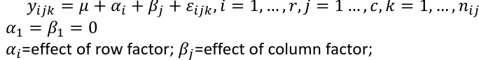

We test different models using ANOVA to look at the global effect of the factors

Sum of Squares

The traditional one-way ANOVA uses a decomposition of the sum of squares for analysis.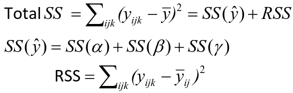

Each sum of squares uses a number of degrees of freedom, given by number of different levels - 1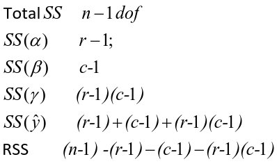

SS(y) = model SS = SS(a) + SS(b) + SS(g)

These sum of squares are computed sequentially, so the order of terms in the model matters! If the design is balances the order does not matter.

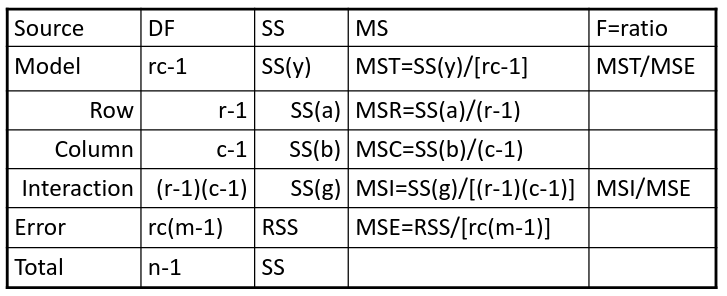
Steps

1. Goodness of fit/Global null hypothesis
   H₀: All parameters = 0
   H_a: At least one differs from 0
2. Test interaction
   • F test is MSI/MSE ~ F_{(r-1)(c-1), rc(m-1)}
   • The P-value is p(F_{(r-1)(c-1), rc(m-1)} > F | H0)
   • If the p-value is smaller than our alpha then we reject the null
   • If we do not reject the null, there is no evidence that all interaction terms are not 0. Fit an additive model and repeat
3. Test main effects
   • If we accept the null hypothesis of no interaction, it makes sense to test the significance of the main effects, to do this we pool the RSS with SS(y)
   • SS(a) and SS(b) are Type III sum of sqaures

Once a model is accepted one can do mean comparisions to identify the factor levels with different effects (Tukey's).

The balance design means the the design is orthogonal and so there is no need to recompute sum of squares or estimates for different models. If not, analyze the data as a traditional linear model.

Problems

When the design is orthogonal/balanced the decomposition SS(a) + SS(b) + SS(g) is unique, when it is not the decomposition depends on the order.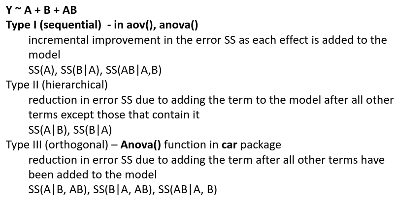

R Code

####### Two-way ANOVA
##### drug dataset
drug <- read.csv("anova.csv", header=T)
drug

hbf <- c(t(drug[,3:5]))
SNP <- c(rep("No",12), rep("Yes", 12))
Drug <- c(rep(0,3), rep(10,3), rep(20,3), rep(30,3),
               rep(0,3), rep(10,3), rep(20,3), rep(30,3))
data.drug <- data.frame(hbf,SNP, Drug)
head(data.drug)

### summaries
overall.mean <- mean(hbf); overall.mean
drug.means <- tapply(hbf, Drug, mean); drug.means
snps.means <- tapply(hbf, SNP, mean); snps.means
cell.means <- tapply(hbf, interaction(Drug,SNP), mean); cell.means

dim(cell.means) <- c(4,2); cell.means
cell.means <- data.frame(cell.means)
row.names(cell.means) <- levels(factor(Drug))
names(cell.means) <- levels(factor(SNP))
cell.means 

## Visualization
#install.packages("gplots")
library(gplots)
plotmeans(hbf~Drug, data=data.drug,xlab="Drug", 
		ylab="HbF",  main="Mean Plot\n with 95% CI")
plotmeans(hbf~SNP, data=data.drug,xlab="SNP", 
		ylab="HbF",  main="Mean Plot\n with 95% CI")
plotmeans(hbf~interaction(Drug,SNP), data=data.drug,
		xlab="SNP",  connect=list(1:4,5:8),ylab="HbF", 
          	main="Interaction Plot\nwith 95% CI")

interaction.plot(factor(Drug), factor(SNP), hbf, type="b",  
		xlab="Drug", ylab="hbf", main="Interaction Plot")


### two-way anova with balanced design
mod <- aov(hbf~as.factor(Drug)*SNP, data=data.drug)
summary(mod)
table(mod$fitted.values)

# TukeyHSD(mod)
mod <- lm(hbf~as.factor(Drug)*SNP, data=data.drug)
summary(mod)
anova(mod)
table(mod$fitted.values)

##### Exercise with balance design

mod.a <- aov(hbf~as.factor(Drug)*SNP, data=data.drug)
summary(mod.a)		# anova(mod.a)
mod.lma <- lm(hbf~as.factor(Drug)*SNP, data=data.drug)
anova(mod.lma)

mod.b <- aov(hbf~SNP*as.factor(Drug), data=data.drug)
summary(mod.b)		# anova(mod.b)
mod.lmb <- lm(hbf~SNP*as.factor(Drug), data=data.drug)
anova(mod.lmb)


##### Exercise with unbalance design
data.drug.1 <- read.csv("data.drug.1.csv", header=T)
mod.1a <- aov(hbf~as.factor(Drug)*SNP, data=data.drug.1)
summary(mod.1a)
mod.1lma <- lm(hbf~as.factor(Drug)*SNP, data=data.drug.1)
anova(mod.1lma)


mod.1b <- aov(hbf~SNP*as.factor(Drug), data=data.drug.1)
summary(mod.1b)
mod.1lmb <- lm(hbf~SNP*as.factor(Drug), data=data.drug.1)
anova(mod.1lmb)