Generalized Linear Models
BS853: Analysis of the quantitative and quantitative data types often found in health science research
- Introduction
- Models for Two-Way Contingency Tables
- Three-Way Contingency Tables
- Binomial Outcomes
- Hypothesis Testing with GLM
- GLM for Multinomial Outcomes
- GLM for Count Data
- Gamma Regression
- Survival - Time to Failure
- GLM for Correlated Data
Introduction
Generalized linear models are extensions of classical linear models. Classes of generalized linear models include linear regression, logistic regression for binary and binomial data, nominal and ordinal multi-nomial logistic regression, Poisson regression for count data and Gamma regression for data with constant coefficient of variation.
Generalized Estimating Equations (GEE) provide an efficient method to analyze repeated measures where the normality assumption does not hold.
Review
Linear Models
Classical linear models are great, but are not appropriate for modeling counts or proportions.
In SAS there are > 10 procedures that will fit a linear regression, example:
title " Simple linear regression of Income " ;
proc reg data = IM ;
model Inc = EN Lit US5 ;
output out = OutIm ( keep = Nation LInc Inc En Lit US5 r lev cd dffit )
rstudent = r h = lev cookd = cd dffits = dffit ;
run ;
quit ;
A model generally fits well if the residuals, or difference between predicted and observed, are small. The assumption of a linear model are primarily checked through the residuals (normality, homoscedasiticity/constant variance and linearity)
Normality assumption of the outcome is almost always not met in real data. One of the solutions proposed is to transform the data. The most popular methods is logarithmic.
Recall that:
Mean(g(Y)) != g*Mean(Y)
GoF and Outliers
R-Squared is a measure of goodness-of-fit where higher values are indicative of a better fit. R2 = Explained Variation / Total Variation
The issue with R-Squared is that more predictors will increase R2 regardless of the quality of the predictor. R-Squared-Adjusted penalizes for complexity.
We do not want observations that lie on the '1%' ends of the distributions to influence the model. The leverage of an observation is defined in terms of its covariate values.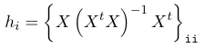
An observation with high leverage may or may not be influential; Where we have p predictors and n observations we define leverage points as hi > 4/n
A point with high leverage might not have high influence, that is the model does not change substantially when the point is excluded. Cook's distance can be used to identify influential points: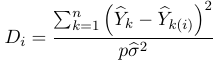 OR
OR 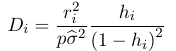
Other measures of the influence are:
DFFITTS, how much an observation has effected the fitted value: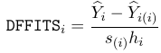
DFBETAS, the difference in each parameter estimate: Values larger than 2/sqrt(n) should be investigated.
Model Selection
Types of models:
- Complete/Full - Reproduces data without simplification; As many parameters as observations
- Null/Intercept - Only the intercept, one predicted value for all observations
- Maximal - largest model that we are prepared to concider
- Minimal - contains minimal model parameters that must be present
- Log-Likelihood ratio statistics
- LRi = 2[log L (Saturated Model) - log Li
- Alike information criterion
- AICm = -2 ln Lm + 2km
- Bayesian Information Criterion
- BICm = -2 ln Lm + km * ln n
Generalized Linear Models
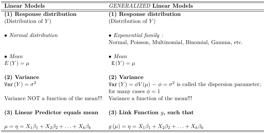
With the Generalized Linear Models, the classic linear model is generalized in the following ways:
- Drops the normality assumption
- Allows the variance of the response to vary with the mean of the response through a variance function
- The mean of a population is allowed to depend on the linear combination of the predictors through a link function g, which could be nonlinear. Shown as:
η = g(μi) = β0 + β1 Xi + β2Xi2+ β3 Xi3
and η is called the linear predictor
With Generalized Linear Models, the classical Linear Model is generalized in a number of ways and is, therefor, applicable to a wider range of problems.
Models for Two-Way Contingency Tables
Recall in the last section Generalized Linear Models (GLMs) were introduced as an extension of the traditional linear model, it eases the assumptions in the following ways:
- Drops the normality assumption
- The response variable is allowed to follow any distribution of the exponential family (binomial, Poisson, negative minomial, gamma, multi-nomial, etc
- Assumes the variance of the response depends on a function of the mean, called a variance function
- The mean of the population is allowed to depend on the linear combination of the predictors through a link function, g
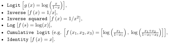
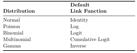
- The following link functions are used most often

- The below table specifies which function to use with each distribution

- The following link functions are used most often
In SAS
- PROC GENMOD
- The GENMOD is a procedure for analyzing generalized linear modes
- PROC LOGISTIC
- The LOGISTIC procedure is constructed for logistic regression and provides useful information
as diagnostic plots, odds ratios and other measures specific to logistic regression models.
- The LOGISTIC procedure is constructed for logistic regression and provides useful information
- PROC CATMOD
- The CATMOD procedure is a procedure designed to fit models to functions of categorical response variables.
All of these procedures report the deviance. PROC LOGISTIC reports AIC and BIC, and it can be calculated with information from PROC CATMOD.
Estimation in Generalized Linear Models
GLMs are estimated with the Maximum Likelihood (ML) method. This chooses the value which makes the observed data the most probable (equivalent to the least squares method).
Example: Let τ be the prevalence of a disease in some population. Suppose that a random sample of size 100 is selected and we observe Y = 40 individuals with the disease.
Use the data(Y) to obtain an estimate of τ_hat(Y), assuming τ has good statistical properties. By "good" it means the estimate has little to no bias and small variance.
In this example, if τ = .5 then we would write the likelihood function as:
Pτ (Y = 40) = 100C40 .540 (1 - .5)100 - 40
As a function of τ, the function Pτ(Y = ?) is called the likelihood function
Log-linear Models/Contingency Tables
Log linear models for contingency tables specify how the cell counts depend on the levels of categorical variables defining that table. Loglinear models treat all variables as symmetrically and attempt to model all important associations among them. In this sense, it's very similar to correlation analysis of continuous variables where the goal is to determine the patterns of dependence and independence among a set of variables.
Loglinear models are generalized linear models with Poisson response distribution, Log link function, and Identify variance function (for Poisson: Expected value = variance)
Data are represented in contingency tables as cell counts. The counts in the cells are assumed to follow a Poisson distribution. Loglinear models are used to model association patterns among categorical variables.
Log linear models are analogous to correlation analysis for normally distributed data, and are most appropriate when there is no clear distinction between response and explanatory variables.
Example of Contingency tables:
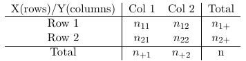
Data can be through of arising by sampling from a population and classify each individual in one of the cell of the two-way cross-classification of the two binary responses it falls in. Each count is assumed to follow a Poisson distribution with expected frequencies: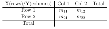
If we fix n (condition on n) the counts in the four cells follow a multinomial distribution.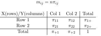
Loglinear models are constricted using the expected values (mij) rather than piij. The main distributional assumption is that nij follow a Poisson distribution with expectancy mij.
There are several different kind of loglinear models we can fit to the data above.
Saturated Model
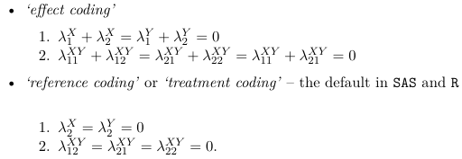
A model that is as complicated as the number of observations. Such a model is over-specified ('less-than-full-rank-coding' or 'GLM coding'). The result does not reduce the complexity of the data and will give a 'perfect prediction'.
The {λX i } are called row effects, {λYj} are called column effects and { λij XY } are called interaction effects.
To solve a saturated model, the practice is to impose linear constraints on the parameters to reduce the number of parameters.
Testing Goodness of Fit in Loglinear Models
As with any other model, the GoF can be evaluated by comparing the observed to the predicted values - or the current model to the saturated model. It is not always appropriate to simply subtract the observed and fitted values!
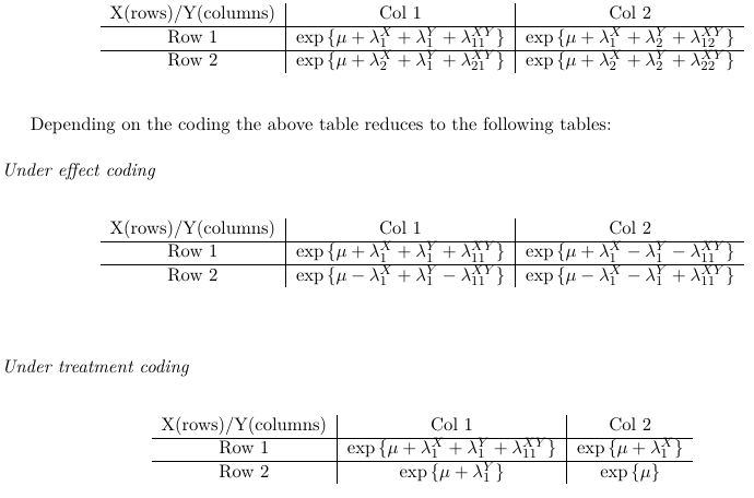
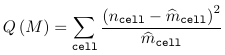
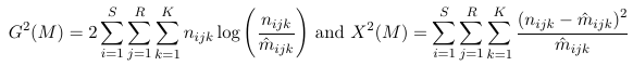
For a loglinear model, two goodness of fit statistics are commonly used:
- Deviance Statistic

- Pearson chi-sqaured statistic

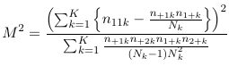
Where ncell is the observed count for a cell and m_hatcell is the fitted cell frequency in model M. Under the assumption that model M is the right model, both G2(M) and Q(M) ~ chi2(n - p), with p being the number of parameters in the model M.

Properties of the Goodness of Fit Statistic
- When the model M holds, both statistics follow a chi-squared with the degrees of freedom equal to the number of cells minus the number of estimated parameters
- The deviance (likelihood ratio) statistic can be used to test the difference between two nested models, M1 and M2
Model M1 is said to be nested in M2 (M1 ⊂ M2) if the parameters are a subset of the parameters in M2.
- The statistic G2(M1 | M2) = G2(M1) - G2(M2) will follow a chi-squared with p2 - p1 DF where p1 and p2 are the number of linearly independent parameters in models M1 and M2, respectively
Saturated Loglinear Model for SxR Table

As above, the {λi^X } are called row effects, {λj^Y} are called column effects and λij^ XY are called interaction effects.
The number of parameters in the above model will be 1 + S + R +RS. The number of observations is S*R, hence the model is over-specified. To reduce the number of parameters linear constraints are imposed on the parameters. For example, reference coding would be represented as:
λSX = λRY = 0, or
λSjXY = λiRXY for every i and j, or:![]()
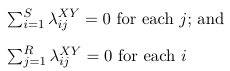
With either of these two coding constraints, the effective number of parameters for the saturated model is:
1 + (S - 1) + (R - 1) + (R - 1)(S - 1) = SR
For any number of dimensions the number of parameters in the saturated log-linear model equals the number of cells in the table. The saturated model give "perfect prediction" since it has the same number of observations as parameters.
Three-Way Contingency Tables
In studying the association between two variables we should control for variables that may influence the relationship. To do so we can create K strata to control for a third variable.
When all involved variables are categorical, we can display the distribution of (E, D) as a contingency table at different levels of C.
The cross-section of tables are called partial tables. The 2-way table that displays the distribution of (E,D) disregarding C is called the E-D marginal table.
Partial tables can exhibit different association than the marginal tables (Simpson's Paradox); for this reason analyzing marginal tables can be misleading.
Simpson's Paradox occurs when an association between two variables is reversed upon observing a third variable.
Independence
In 1959, Mantel and Haenszel proposed a test for independence (between E and D) while adjusting for a third variable (C). This test statistic is called the Cochran-Mantel-Haenszel test statistic and is defined as:
1. Under the conditional independence assumption (across all strata) M2 follows a chi-squared distribution with 1 degree of freedom.
2. M2 has good power against the alternative hypothesis of consistent patterns of association across strata.
If conditional independence assumption fails one might be interested in testing the assumption that OR is the same across the K tables. This could be done with the Breslow-Day Test for Homogeneity of Odds Ratios (reported by PROC FREQ in SAS).
title1 " Care and Infant survival in 2 clinics " ;
data care ;
input clinic survival $ count care ;
cards ;
1 died 3 0
1 died 4 1
1 lived 176 0
1 lived 293 1
2 died 17 0
2 died 2 1
2 lived 196 0
2 lived 23 1
run ;
proc freq data = care ;
table clinic * survival * care / cmh chisq relrisk ;
weight count ; run ;
Note that:
- The methods outlined here apply not only to situations where the classification variables are both responses (this will be explored in a later section)
- We will cover a way to test conditional independence based on Log-Linear models next
Log-Linear Models for S x R x K Tables
Every association between three variables can be coded with a different Log-Linear model. We will select among the association patters, using the deviance GoF statistic.
Saturated Model

The number of parameters: 1 + S + R + K + RK + SK + RSK
To reduce the number of parameters we impose linear constraints on the parameters. Consider the following examples:
Reference Coding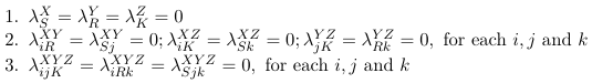
Effect Coding (Zero Sum Constraints)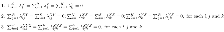
In the saturated model the number of parameters is:
1+(S - 1)+(R - 1)+(K −1)+(S −1)(R−1)+(S −1)(K −1)+(R−1)(K −1)+(S −1)(R−1)(K −1) = SRK
Note that with the saturated model we make no assumption regarding the association among variables.
All Two-Way Interaction Model
Let's consider another model with all two-way interactions (no three-factor interaction):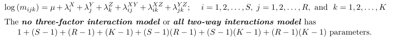
Under this model the association between X and Y is the same between different levels of Z; The association between X and Z is the same at different levels of Y; and the association between Z and Y is the same at different levels of X.
We can actually do the math and o serve that the Odds Ratio between X and Y (ORKXY) is the same at all levels of Z (it does not depend on k):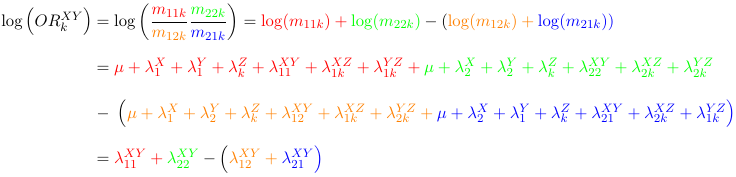
Mutual Independence Model

No interactions, the model assumes X, Y and Z are mutually independent.
The number of parameters will be: 1 + (S - 1) + (R - 1) + (K - 1)
Again, here the partial and marginal odds ratio between X and Y is 1 and does not depend on the level of Z.
Conditional Independence Models
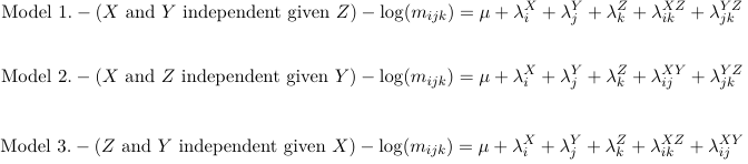
Model 1 will have number of parameters: 1 + (S − 1) + (R − 1) + (K − 1) + (S − 1)(K − 1) + (R − 1)(K − 1)
Joint Independence Models
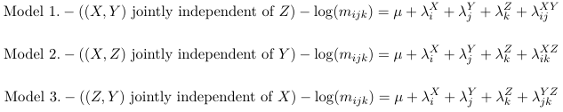
With the first having number of parameters: 1 + (S − 1) + (R − 1) + (K − 1) + (S − 1)(R − 1)
Graphs
Each of these models is hierarchical and can be represented by a association graph. This is a graph which represents which variables are independent, conditionally independent or associated.
The number of vertices is equal to number of variables, and edges represent partial association between he corresponding variables.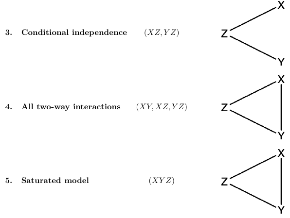
Modeling Strategy
- Model Selection
- The likelihood ratio statistics can be broken down conditionally; Given two nested models the G2(M2 | M1) = G2(M2) - G2(M1), measures the additional contribution to the fit of the model M1 over M2 and (under the assumption M2 holds) will follow a chi-square distribution with p1 - p2 df

- Use all your subject matter knowledge searching for the best model
- The number of models that should be considered increases exponentially with number of parameters
- One strategy is to first compare independence (interaction and saturation model); Then identify the simplest model in between this model and the nested model.
- The test statistics are independent and one should adjust the significance level for multiple testing.
- The likelihood ratio statistics can be broken down conditionally; Given two nested models the G2(M2 | M1) = G2(M2) - G2(M1), measures the additional contribution to the fit of the model M1 over M2 and (under the assumption M2 holds) will follow a chi-square distribution with p1 - p2 df
- Occam's razor pinciple (All things being equal, the simplest solution tends to be the best one) - If the difference in Likelihood ratios is not significant, choose the more parsimonious model
- Structural zero cells are cells for which it is impossible to have a count greater than 0; These should be treated differently than 0s that happen by design (Sampling Zeros). One practice is to add a small constant (.0001).
Higher Dimension tables
Three way tables are significantly more complicated than two-way tables due to the fact that the number of interaction terms increases and the possible association among variables increases. With higher dimension tables, the number of cells increase exponentially. This creates problems with inferences as we require a larger data set in which some cases might not be available. If the data does exist though, then we can use the same strategy for model fit and selection.
SAS Code
data THR ;
input Rural Income Satisf Count ;
datalines ;
1 1 1 48
1 1 2 12
1 2 1 96
1 2 2 94
2 1 1 55
16
BS853 - Generalized Linear Models
 Spring 2023
2 1 2 135
2 2 1 7
2 2 2 53
run ;
title1 ’ Association among residence , income and satisf with total hip replacement ( THR ) ’;
options ps =60 ls =89 pageno =1 nodate ;
title2 ’ Model 1 saturated model ’;
ods select ModelFit ;
proc genmod data = THR ;
class Rural Income Satisf ;
model count = Rural | Income | Satisf / dist = poissonrun ;
obstats type3 ;
title2 ’ Model 2 - all two - way interactions ’;
ods select ModelFit ;
proc genmod data = THR ;
class Rural Income Satisf ;
model count = Rural | Income Rural | Satisf Satisf | Income / dist = poisson obstats type3 ;
run ;
title2 ’ Model 3 - conditional independence of Income and Rural ’;
ods select ModelFit ;
proc genmod data = THR ;
class Rural Income Satisf ;
model count = Rural | Satisf Satisf | Income / dist = poisson obstats type3 ;
run ;
title2 ’ Model 4 - conditional independence of Satisfaction and Rural ’;
ods select ModelFit ;
proc genmod data = THR ;
class Rural Income Satisf ;
model count = Rural | Income Satisf | Income / dist = poisson obstats type3 ;
run ;
title2 ’ Model 5 - conditional independence of Satisfaction and Income ’;
ods select ModelFit ;
proc genmod data = THR ;
class Rural Income Satisf ;
model count = Rural | Income Rural | Satisf / dist = poisson obstats type3 ;
run ;
title2 ’ Model 6 - joint independence of ( Income and Satisfaction ) from Rural ’;
ods select ModelFit ;
proc genmod data = THR ;
class Rural Income Satisf ;
model count = Rural Satisf | Income / dist = poisson obstats type3 ;
run ;
title2 ’ Model 7 - joint independence of ( Income and Rural ) from Satisfaction ’;
ods select ModelFit ;
proc genmod data = THR ;
class Rural Income Satisf ;
model count = Rural | Income Satisf / dist = poisson obstats type3 ;
run ;
title2 ’ Model 8 - joint independence of ( Rural and Satisfaction ) from Income ’;
ods select ModelFit ;
proc genmod data = THR ;
class Rural Income Satisf ;
model count = Rural | Satisf Income / dist = poisson obstats type3 ;
run ;
title2 ’ Model 9 - Mutual independence of Income , Rural , and Satisfaction ’;
ods select ModelFit ;
proc genmod data = THR ;
class Rural Income Satisf ;
model count = Rural Satisf Income / dist = poisson obstats type3 ;
run ;
Binomial Outcomes
Frequently dichotomous outcomes are used in medical studies, such as presence of a disease or exposure to some factor. The classical model does not apply outcomes that are not continuous, and many other reasons:
- The variance of the dichotomous response is not constant
- One could predict probabilities > 1 or smaller than 0
- Limited interpretation of parameters
In this section we will observe alternatives to traditional linear regression for binomial data.
Generalized Linear Model For Binomial Data
- The outcome is distributed either Bernoulli or Binomial with probability of success θ
- Link function is logit and relates to the probability of success θ to the linear predictor η = β0 +β1 X1 +
β2X2 + · · · + βk−1Xk−1 + βk Xk as follows:

- Variance function: V(θ) = θ (1 - θ)

Recall: For ordinary linear regression the distribution of outcomes is normal and the link is the identity function, and the variance is constant. For loglinear models the distribution of the outcome is Poisson, the link function is the LOG function and the variance function is the identity.
The link function is logistic because the logit function takes value between -inf to inf while the logodds is between 0 and 1.
β represents the increase in logodds for a one-unit increase in X
The coefficients can also be interpreted as probability (risk) difference. However, the change is a function of base probability:
Probit, Complementary Log-Log, and Logistic Regression
Probit regression and Complementary log-log regression are generalized linear models for the same type of data as the logistic regression, the only difference is in the choice of the link functions.
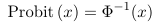
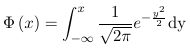
- Probit uses a link function which is the inverse of the Cumulative Distribution Functions (CDF) of a standard normal distribution
- Link function:

Where
- Probit and logistic will in general give similar results in terms of significance; The advantage of logistic regression is interpretability of coefficients as OR's
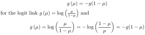
- Logit and Probit haave the symmetry property, that is:

- Link function:
- Complementary log-log is inverse of the CDF for an extreme value distribution
- The link function:

- Does not have the symmetry property, a good choice when symmetry property does not hold.
- The link function:
Interpretation of Parameters
Note we've already seen how to interpret logodds in 806 and 852 so I will not being going into great detail here.
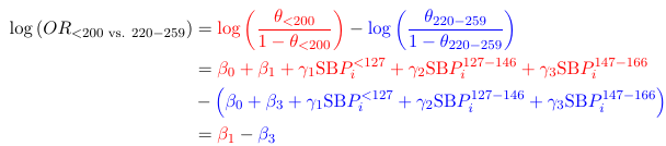
One neat thing is that we can express any model using shorthand. 
Where CHOL and SBP are binary variables representing levels of these measures. The shorthand equivalent: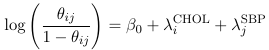
While not as informative about the levels and coefficients, it is much easier to write.
Testing GoF and Model Selection
As in any other model we can assess the GoF by comparing the observed to the predicted. The deviance statistic (also called the Likelihood Ratio Statistic) is the GoF measure of choice for this class. It can be used to compare any nested model, and since every model is nested within the saturated model, we can use:
Which reduces to the following for binomial models: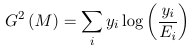
Where Ei = ni πi
The Pearson Chi-Squared Test are application for logistic regression when the data can be aggregated, or grouped into unique profiles determined by predictors. Aggregation is only possible when all predictors are categorical.
With ungrouped data the Pearson chi-square test is: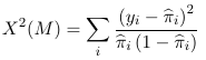
Where yi is the observed binary outcome, and pi_hat is the model estimate of probability of yi=1. This does NOT have a asymptotic chi-square distribution, but when properly standardized it follows a normal distribution
With grouped data the Pearson chi-square test is: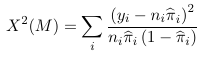
which follows a chi-square distribution
Note that when all independent variables are categorical, a logistic regression can be estimated using a suitably formulated loglinear model - the converse is NOT always true.
Hosmer-Lemeshow GoF Test
The probabilities of the event are estimated using the model for each unit in the data as: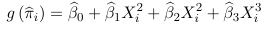 or
or ![]()
Where β parameteres are estimated by maximum likelihood. These predicted values are then compared with the observed values of Y (which is binary)
The HL test is based on ordering the sample according to the risk or predicted probability. The estimated probabilities are split into 10 groups (by default), the first group consists of the 10% lowest estimated probabilities and so on.Based on the observed Yi's we can calculate the the number of Yi's equal to 0 or 1 in each group.
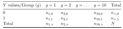
To estimate the number of 1's and 0's expected base on the model, we calculate the average of the estimated probabilities in each group and multiply by the number of observations per group.
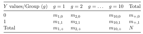
The Hosmer-Lemshow test is a Pearson chi-squared statistic comparing the two tables: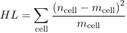
In the original 1980 paper HL showed the test statistic followed a ~chi-squared distribution with 10 - 2 = 8 degrees of freedom. A small p-value indicates poor fit.
Criticisms
- The HL test could depend on the number of groups/choosing a different number of groups can yield different results
- The suggested number of groups is dependent on the number variables in the model, that is #predictors + 1
Measuring Predictive Ability
There are several measures for quantifying prediction ability in logistic regression. The first set of measures below is based on maximum likelihood values and can be used for any likelihood based models. There are measures specific to models with multi-nomial outcomes.
Maximum Likelihood Based Measures
- L* = -2 * LL ; Minus twice the maximum log-likelihood of the saturated model (lowest possible value)
- L = -2 * LL ; Minus twice the maximum log-likelihood of the current model
- L0 = -2 * LL ; Minus twice the maximum log-likelihood of the model including only intercept
The deviance is a test for the significance of all predictors in addition to the intercept:
LR = L0 - L
The largest value that can be explained by a model:
LR = L0 - L*
The fraction that is explained from what can by explained is:
R2 = (L0 - L) / (L0 - L*) = LR / (L0 - L*)
Which is the same as R2 from linear regression. However, this statistic has some undesirable properties, to circumvent these RLR2 has been proposed as: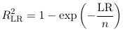
Which is how SAS calculates RSQUARE in proc logistic; And adjusted R2: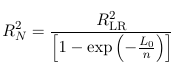
Other measures:
- c-statistic or Area Under Curve (AUC) with a value close to 1 indicating good prediction ability while a value close to .5 indicates a poor predictive ability. Closely related to Mann-Whitney, Wilcoxon statistics and the Gini Coefficient
- Somers' D statistic DXY = 2(c - .5) rank correlation with a value close to 1 indicating good prediction ability
- Recent of correctly classified responses
Adjusting for Optimism (Bias) In Measures of Predictive Ability
When the same dataset is used to fit the model and assess its predictive ability it can result in a 'optimistic' estimate of predictive ability. There are a number of approaches to adjust these estimates including: data splitting, cross-validation and bootstrapping.
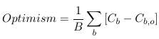
Using Bootstrap to Estimate Optimism
Bootstrapping is a generic and efficient approach in statistics. It involves repeatedly sampling with replacement from the observed dataset. This process can be repeated to create many (say B) bootstrap datasets. The fundamental principle at work is that the original observed data are a good approximation on what the population on the whole of interest is, and then the bootstrap data set represent instances of data samples from that population.
- Fit model to original data, and estimate C0
- Obtain B bootstrap data as indicated above; For each:
- Fit the model to the bootstrap datasets and estimate Cb
- Estimate the c-statistic of the model in 2a. on the original data to be Cb,0
- Since the model in 2a was estimated on bootstrap data it is expected that Cb,0 < Cb, estimate the optimism as:

- Estimate the corrected c-statistic as C0 - Optimism
This approach for correcting the measure of predictive ability is very general and applies to all the measures presented above. The ideal estimate of predictive ability of a model is obtained on an independent sample.
SAS Code
options ps=60 ls=89 pageno=1 nodate;

/* CHD in Framingham Study*/
proc format ;
value sbp 1='<127' 	2='127 - 146' 	3='147 - 166' 	4='167+';
value chl 1='<200'  2='200 - 219'   3='220 - 259'   4='>=260';
run;
data chd;
input Chol SBP CHD Total;
prchd=(chd+0.5)/total;
logitp=log((prchd)/(1- prchd));
format sbp sbp. Chol chl.;
cards;
1 1 2  119
1 2 3  124
1 3 3  50
1 4 4  26
2 1 3  88
2 2 2  100
2 3 0  43
2 4 3  23
3 1 8  127
3 2 11 220
3 3 6  74
3 4 6  49
4 1 7  74
4 2 12 111
4 3 11 57
4 4 11 44
;
run;


/* First, examine the relationships of incidence of CHD with Chol and SBP graphically. */
goptions reset=all ftext='arial' htext=1.2 hsize=9.5in vsize=7in aspect=1 horigin=1.5in vorigin=0.3in ;
goptions device=emf rotate=landscape gsfname=TempOut1 gsfmode=replace;
  		filename TempOut1 "C:\Documents and Settings\doros\My Documents\Projects\BS853\Class 4\Framingham.emf";
axis1 label=(h=1.5 'Cholesterol') minor=none order=(1 to 4 by  1)
value=(tick=1 '< 200' tick=2 '200 - 219' tick=3 '220 - 259' tick=4 '>= 260') offset=(1);
axis2 label=(h=1.5  a=90 'Logit(Probability)') minor=none ;

symbol1 v=none i=j ci=red line=1;
symbol2  v=none i=j ci=green line=2;
symbol3  v=none i=j ci=blue line=3;
symbol4  v=none i=j ci=magenta line=4;
title1 'Incidence of CHD with Chol and SBP';
proc gplot data=chd;
 plot logitp*chol=sbp/haxis=axis1 vaxis=axis2;
 run;
quit;
goptions reset=all;

/* Fit different Models using GENMOD and LOGISTIC*/
options ls=100 ps=60 nodate pageno=1;
title1 'Only Intercept Effect';
proc genmod data=CHD;
class CHOL SBP;
model CHD/Total=/dist=Binomial link=logit;
run;

title1 'Only Chol Effect';
proc genmod data=CHD;
class CHOL SBP;
model CHD/Total=CHOL /dist=Binomial link=logit;
run;

title1 'Only SBP Effect';
proc genmod data=CHD;
class CHOL SBP;
model CHD/Total=SBP /dist=Binomial link=logit;
run;


title1 'Only main Effects';
ods output obstats=check;
proc genmod data=CHD;
class CHOL SBP;
model CHD/Total= CHOL SBP /dist=Binomial link=logit obstats;
run;

title1 'Only main Effects - Using PROC LOGISTIC';
proc logistic data=CHD;
class CHOL SBP(ref='167+');
model CHD/Total= CHOL SBP ;
run;

title1 'Only main Effects - Continuous predictors';
ods output obstats=check;
proc genmod data=CHD;
model CHD/Total= CHOL SBP /dist=Binomial link=logit obstats ;
run;

title1 ' Saturated Model ';
proc genmod data=CHD;
class CHOL SBP;
model CHD/Total= CHOL|SBP /dist=Binomial link=logit;
run;

title1 'Only main Effects - Hosmer-Lemeshow';
ods select LackFitPartition LackFitChiSq;
proc Logistic data=CHD;
  model CHD/Total= CHOL SBP / LACKFIT;
run;

title1 'Only main Effects - R-Squared and R-Squared Nagelkerke';
ods select RSQUARE;
proc Logistic data=CHD;
  model CHD/Total= CHOL SBP / RSQUARE;
run;

 /* Logistic regression models as Log-Linear models*/
data chd2;
input chol sbp chd count @@;
datalines;
1 1 1 2  1 1 2 117
1 2 1 3  1 2 2 121
1 3 1 3  1 3 2  47
1 4 1 4  1 4 2  22
2 1 1 3  2 1 2  85
2 2 1 2  2 2 2  98
2 3 1 0  2 3 2  43
2 4 1 3  2 4 2  20
3 1 1 8  3 1 2 119
3 2 1 11 3 2 2 209
3 3 1 6  3 3 2  68
3 4 1 6  3 4 2  43
4 1 1 7  4 1 2  67
4 2 1 12 4 2 2  99
4 3 1 11 4 3 2  46
4 4 1 11 4 4 2  33
;
title1 'Logistic regression models as Loglinear models';
title2 'Model 1' ;
ods select parameterestimates modelfit;
proc genmod data=chd2;
class chol sbp chd;
model count=CHD SBP|CHOL /link=log dist=poisson obstats;
run;

ods select parameterestimates modelfit;
title2 'Model 2' ;
proc genmod data=chd2;
class chol sbp chd;
model count=CHD|SBP SBP|CHOL/link=log dist=poisson obstats;
run;

ods select parameterestimates modelfit;
title2 'Model 3' ;
proc genmod data=chd2;
class chol sbp chd;
model count=CHD|CHOL SBP|CHOL/link=log dist=poisson obstats;
run;
options ls=90;
ods select parameterestimates;* modelfit;
title2 'Model 4' ;
proc genmod data=chd2;
class chol sbp chd;
model count=CHD|CHOL CHD|SBP SBP|CHOL/link=log dist=poisson obstats;
run;

/**************************************************************/
/* Admission Data                                             */
/**************************************************************/
/* Ignoring Department */
data overall;
input sex $ yes total;
cards;
	M 1198  2691
	F   557  1835
;
/* Saturated model: with class statement*/;
ODS select modelfit ParameterEstimates;
title 'Differential admission by Gender';
proc genmod data=overall;
class sex;
model yes/total=sex/link=logit dist=bin obstats;
estimate 'overall gender' sex 1 -1/exp;
run;

proc genmod data=overall;
class sex;
model yes/total=/link=logit dist=bin obstats;
run;
/* By Department */
data one;
do Department=1 to 6;
do Sex='M', 'F';;
input yes no;
logitp=log(yes/(yes+no));
total=yes+no;
output;
end;
end;
cards;
512	313
89	19
353  	207
17     	8
120  	205
202  	391
138  	279
131 	244
53  	138
94  	299
22  	351
24  	317
;run;

/* Explain why marginally women seem to be discriminated against
   - More women apply to harder to enter colodges!!!             */

proc sql; create table a as
select department, sum(total) as total , sum(yes)/sum(total) as adminp from one group by department  order by department;
 create table b as select department, total as fem from one where sex='F' order by department;
 create table c as
 select *, fem/total as pf from a as aa, b as bb where aa.department=bb.department;
quit;

 symbol1 v=circle i=join;
 proc gplot data=c;
 plot pf*adminp;
run;


goptions reset=all ftext='arial' htext=1.2 hsize=9.5in vsize=7in aspect=1 horigin=1.5in vorigin=0.3in ;
goptions device=emf rotate=landscape gsfname=TempOut1 gsfmode=replace;
  		filename TempOut1 "C:\Documents and Settings\doros\My Documents\Projects\BS853\Class 4\admission.emf";
		symbol1 v=dot i=j ci=red;
		symbol2 v=circle i=j ci=blue;
		axis1 label=(h=1.5 'Department') minor=none order=(1 to 6 by  1)  offset=(1);
axis2 label=(h=1.5  a=90 'Logit(Rate)') minor=none ;

title1 'Admitance by Department and Sex';
proc gplot data=one;
plot logitp*Department=sex/vaxis=axis2 haxis=axis1;
run;

title1 'Saturated Model';
proc genmod data=one;
class department sex;
model yes/total=sex|department/dist=b link=logit;
run;

title1 'Only main effects Model';
proc genmod data=one;
class department sex;
model yes/total=sex department/dist=b link=logit;
run;

title1 'Only Sex Model';
proc genmod data=one;
class department sex;
model yes/total=sex/dist=b link=logit;
estimate 'l' sex 1 -1/exp;
run;

title1 'Only Department effects Model';
proc genmod data=one;
class department sex;
model yes/total=department/dist=b link=logit;
run;

ods select estimates;
title1 'Estimated ODDS Ratio (F vs M) in each Department';
proc genmod data=one;
class department sex;
model yes/total=sex|department/link=logit dist = bin covb;
estimate 'sex1'  sex 1 -1  department*sex 1 -1 0  0 0  0 0  0 0  0 0  0    /exp ;
estimate 'sex2'  sex 1 -1  department*sex 0  0 1 -1 0  0 0  0 0  0 0  0    /exp ;
estimate 'sex3'  sex 1 -1  department*sex 0  0 0  0 1 -1 0  0 0  0 0  0    /exp ;
estimate 'sex4'  sex 1 -1  department*sex 0  0 0  0 0  0 1 -1 0  0 0  0    /exp ;
estimate 'sex5'  sex 1 -1  department*sex 0  0 0  0 0  0 0  0 1 -1 0  0    /exp ;
estimate 'sex6'  sex 1 -1  department*sex 0  0 0  0 0  0 0  0 0  0 1 -1    /exp ;
run;

/* Modeling Trends in Proportions */
data refcanc;
do age=1 to 4;
input cases ref;
total=cases+ref;
output;
end;
cards;
26	20
4	7
3	10
1	11
;
run;

/* only intercept */
title1 'Only Intercept model';
proc genmod data=refcanc;
class age;
model cases/total=;
run;

/* Saturated model */
title1 'Saturated model';
proc logistic data=refcanc;
class age;
model cases/total=age;
run;
title1 'Linear trend model';

proc logistic data=refcanc;
model cases/total=age;
run;
Hypothesis Testing with GLM
Effect modification can be modeled with logistic regression by including interaction terms. A significant interaction term implies a departure from heterogeneity between groups.
Consider the following example were we wish to compare admission rates by sex per department: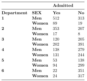
With summary of fit: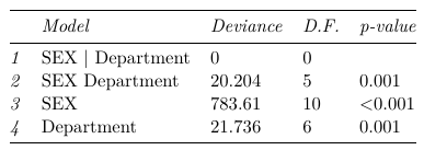
Which we observe only the saturated model fits the data well. To compare ORs across department we estimate the department specific odds from the saturated model:
ods select estimates ;
title1 ’ Estimated ODDS Ratio ( F vs M ) in each Department ’;
proc genmod data = one ;
class department SEX ;
model yes / total = SEX | department / link = logit dist = bin covb ;
estimate ’ SEX1 ’ SEX 1 -1 department * SEX 1 -1 0 0 0 0 0 0 0 0 0 0/exp;
estimate ’ SEX2 ’ SEX 1 -1 department * SEX 0 0 1 -1 0 0 0 0 0 0 0 0/exp;
estimate ’ SEX3 ’ SEX 1 -1 department * SEX 0 0 0 0 1 -1 0 0 0 0 0 0/exp;
estimate ’ SEX4 ’ SEX 1 -1 department * SEX 0 0 0 0 0 0 1 -1 0 0 0 0/exp;
estimate ’ SEX5 ’ SEX 1 -1 department * SEX 0 0 0 0 0 0 0 0 1 -1 0 0/exp;
estimate ’ SEX6 ’ SEX 1 -1 department * SEX 0 0 0 0 0 0 0 0 0 0 1 -1/exp;
run ;
The hypothesis tests we've encountered so far can be expressed in terms of linear combinations of the model parameters; However, other tests have to be carried out that may not be included in default output which requires a good understanding of the model.
For example, a few important properties we've seen so far:
- Differences between groups (Lecture 4)
Expressed as a linear combination:
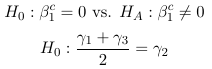
1 × β1 + 0 × β2 + (−1) × β3 + 0 × β4 = 0 - Independence in 2 way tables defines by categorical variables X and Y
H0: X and Y are independent <-> H0: all λXYij = 0
HA: X and Y are dependent <-> HA: at least one λXYij != 0
Expressed as a linear combination:
λ11 = λ12 = λ21 = λ22 = 0
1 × λ11 + 0 × λ12 + 0 × λ21 + 0 × λ22 = 0
0 × λ11 + 1 × λ12 + 0 × λ21 + 0 × λ22 = 0
0 × λ11 + 0 × λ12 + 1 × λ21 + 0 × λ22 = 0
0 × λ11 + 0 × λ12 + 0 × λ21 + 1 × λ22 = 0 - Significance of parameters (Lecture 4)

Expressed as a linear combination:
(For ordinal SBP): 0 × β0c + 1 × β1c + 0 × β2c = 0
(For SBP): γ1 + (−2) × γ2 + γ3 + 0 × γ4 = 0
In all cases the null hypothesis can be expressed as a linear combination of the parameters (this is important in understanding contrast and estimate statements in SAS).
Looking at ex. 1 above, we could test the null hypothesis with a t-test: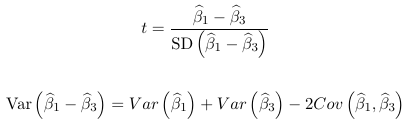
or the Wald test with w = t2. Only variances of coefficients are reported by default in PROC GENMOD, so to get the covariance matrix the covb option is needed in the model statement. But when we want to test more than one linear combination of parameters at the same time this becomes complex and time consuming to do manually.
Within SAS's PROC GENMOD or LOGISTIC we use CONTRAST and ESTIMATE statements to carry out this type of test.
title1 ’ Contrasting <200 vs . 220 -259 with CONTRAST and ESTIMATE statements ’;
proc genmod data = CHD ;
class CHOL SBP ;
model CHD / Total = CHOL SBP / dist = Binomial link = logit ;
estimate ’ <200 vs . 220 -259 ’ CHOL 0 -1 1 0/ exp ;
contrast ’ <200 vs . 220 -259 ’ CHOL 0 -1 1 0;
run ;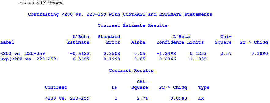
The chi-sqaure test statistic in the two tests is different because estimate uses a t-test while contrast uses a Wald test.
For a categorical variable variable has k levels, the GLM parameterization generates k indicators to
include in the model. For this reason, the GLM parameterization produces a singular model matrix.
Note the following:
- The order of the levels in SAS is critical to outcome.
- The values entered in L, the contrast matrix, must be changed if the parameterization (coding) changes.
- In most procedures the default parameterization is less than the full rank parameterization
- You can alter the default parameterization with the param= option and ordering the levels in the class statement (by using PROC FORMAT)
*Code the categories;
data remission ;
input LLI $ 1 -5
cards ;
8 -12 7 1 1
14 -18 7 1 2
20 -24 6 3 3
26 -32 3 2 4
34 -38 4 3 5
run ;
total remiss grp ;
proc format ;
value $a ’ 8 -12 ’ = ’1 ’ ’ 14 -18 ’= ’2 ’’ 20 -24 ’= ’3 ’ ’ 26 -32 ’= ’4 ’ ’ 34 -38 ’= ’5 ’; run ;

*Here the parameters of interest are the 4th and 5th parameter;
title ’ Default order - Alphanumeric ordering ’;
title2 ’ GLM Coding ’;
ods select classlevels parameterestimates contrasts ;
proc genmod data = remission ;
class LLI ;
model remiss / total = LLI ;
contrast ’ 34 -38 vs . 8 -12 ’ LLI 0 0 0 1 -1;
contrast ’ 34 -38 vs . 8 -12 ’ LLI 0 0 0 1 -1/ wald ;
run ;

*Use format to change the order from 1st to 5th;
title ’ Desired order - Using proc format ’;
title2 ’ GLM Coding ’;
ods select classlevels parameterestimates contrasts ;
proc genmod data = remission ;
format LLI $a .;
class LLI ;
model remiss / total = LLI ;
contrast ’ 34 -38 vs . 8 -12 ’ LLI -1 0 0 0 1;
contrast ’ 34 -38 vs . 8 -12 ’ LLI -1 0 0 0 1/ wald ;
run ;

*We only estimate 4 parameters since the effect of 20-24 is 0 so the 3rd and 4th parameters are of interest;
title ’ Changing Default coding in proc genmod ’;
title2 ’ Change to Reference Coding ’;
ods select classlevels parameterestimates contrasts ;
proc genmod data = remission ;
/* Changed to Reference coding using the ’ param = ref ’ statement . */ ;
class LLI ( ref = ’ 20 -24 ’) / param = ref ;
model remiss / total = LLI ;
contrast ’ 34 -38 vs . 8 -12 ’ LLI 0 0 1 -1;
run ;

*Testing: λ4 − λ5 = λ4 − (−λ1 − λ2 − λ3 − λ4 ) = (1)λ1 + (1)λ2 + (1)λ3 + (2)λ4;
title ’ Changing Default coding in proc genmod ’;
title2 ’ Change to Effect Coding ’;
ods select classlevels parameterestimates contrasts ;
BS853 - Generalized Linear Models
proc genmod data = remission ;
class LLI / param = effect ;
model remiss / total = LLI ;
contrast ’ 34 -38 vs . 8 -12 ’ LLI
run ;

*Comparing the 1st, 4th and 5th parameters;
title1 ’ Two contrasts for multiple hypothesis ’;
ods select pa ra meterestimates contrasts ;
proc genmod data = remission ;
class LLI ;
model remiss / total = LLI ;
contrast ’ 34 -38 vs . 14 -18 vs . 8 -12 ’ LLI 0 0 0 1 -1 , /* ( H01 ) */
LLI 1 0 0 0 -1; /* ( H02 ) */
run ;

*Contrasts involving interactions;
options pageno =1;
title1 ’ OR in each Department for the Saturated Model ’;
ods output estimates = estimates parminfo covB parameterestimates classlevels ;
proc genmod data = one ;
class department SEX ;
model yes / total = SEX | department / link = logit dist = bin covb ;
estimate ’ SEX1 ’ SEX 1 -1 department * SEX 1 -1 0 0 0 0 0 0 0 0 0 0/ exp;
estimate ’ SEX2 ’ SEX 1 -1 department * SEX 0 0 1 -1 0 0 0 0 0 0 0 0/ exp;
estimate ’ SEX3 ’ SEX 1 -1 department * SEX 0 0 0 0 1 -1 0 0 0 0 0 0/ exp;
estimate ’ SEX4 ’ SEX 1 -1 department * SEX 0 0 0 0 0 0 1 -1 0 0 0 0/ exp;
estimate ’ SEX5 ’ SEX 1 -1 department * SEX 0 0 0 0 0 0 0 0 1 -1 0 0/ exp;
estimate ’ SEX6 ’ SEX 1 -1 department * SEX 0 0 0 0 0 0 0 0 0 0 1 -1/ exp;
run ;
Note:
- In PROC LOGISTIC the estimate and contrast statement is implemented exactly the same as above
- If you use the default less-than-full-rank GLM class variable parameterization, each row of the L matrix is checked for estimability. If GENMOD finds a contrast to be non-estimatable it displays missing values in corresponding rows in the results.
- If an effect is not specified in the CONTRAST statement, all of its coefficients in the L matrix are set to 0. If too many values are specified for an effect the extra ones are ignored. If too few are specified, the remaining ones are set to 0.
- For specifying contrasts for interactions, the order you list your categorical variables in the class statement is important
GLM for Multinomial Outcomes
Multinomial outcomes are much akin to binomial outcomes, with added complexity due to outcomes with more than 2 levels. In such cases it can be difficult to determine an 'order' to the outcomes.
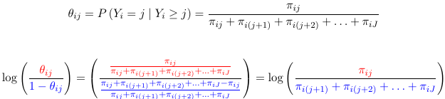
Log-linear models can be used for analysis of this type of data. For example, if we have some distribution where πij represents the probability that the ith individual falls under the jth category. Assuming the response categories are mutually exclusive:
For each individual i; That is the probabilities add up to 1 for each individual, so we only have J - 1 probability parameters.
Multinomial Distribution
This is an extension of the binomial distribution involving joint distributions. Specifically each trial can result in any of the k events (E1, E2 ... Ek), each with its own respective probabilities. The probability that in n trials we observe Y1 of the E1 outcomes, y2 of the R2 outcomes ... and yk of the Rk outcomes in n independent trials is:![]()
with y1 + y1 .. + yk = n and the probabilities summing to 1
The multinomial term: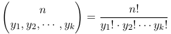
represents the number of possible divisions of n distinct objects into k distinct groups of sizes y1, y2... yk
Consider an example with k = 3 (three possible outcomes):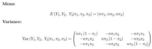
The multinomial distribution model counts are negatively correlated; The dispersion parameter is φ = 1
The binomial distribution can be thought of as a particular case of the multinomial distribution with k = 2. We want models for the mean of the response or equivalently for the probabilities, where the probabilities depend on a vector of covariates.
Link Function - Generalized Logits
Perhaps the simplest approach to the Multinomial regression is to designate one of the response categories as the reference category and calculate the log-odds for all other categories relative to the reference. For the binomial example, the reference cell is often the 'non-event' category.
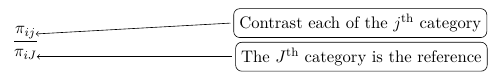
So for a multinomial with J categories there are J - 1 distinct odds. For example, in a case with 3 response categories we could use the last category as the reference and hence get 2 generalized odds also called generalized logits: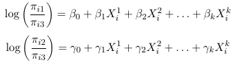
This is kind of like running 2 separate logistic regressions and estimating two separate sets of parameters, but it is a single model and all parameters are estimated by the MLE.
We can solve for the probabilities as a function of the slope parameters (beta and gamma):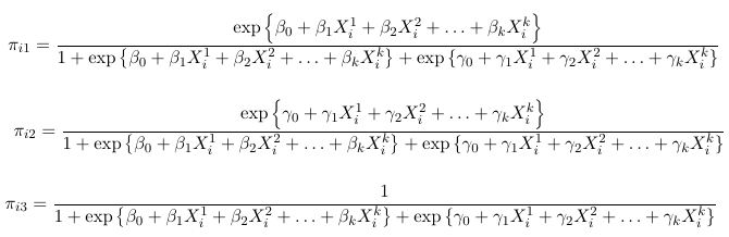
Thus, for a multinomial response with J categories, the J - 1 generalized logits are: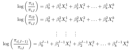
And then maximum likelihood can be used to estimate all parameters. For the intercept and each predictor, we will be estimating J - 1 parameters. Note that it really makes no difference which category is the reference, as we can always convert from one model formulation to another.
Interpretation
The generalized odds of having a response j relative to J are: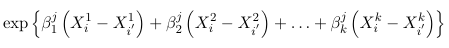
times higher for an individual with characteristics Xi1, Xi2, Xi3... Xik than for a individual with characteristics Xi'1, Xi'2, Xi'3... Xi'k. In particular, keeping X2 through Xk constant for each increase of one unit in X1 the odds of having a response j relative to J changes by a multiplicative factor of exp(beta1j)
Multinomial Ordinal Responses
Consider a multinomial random varaible Yi that may take one of J outcomes, assume there is a natural order from 1 to J. The probability falls into category j or lower is fij = P(Yi <= j), also called the cumulative probabilities.
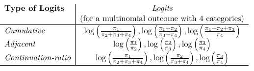
When we have a clear order between categories several alternative regression models are available. We could use generalized logits model but it ignores the order of the levels and this have diminished power. The drawback of multinomial logits compared to general multinomial logits is that assumptions imposed may not be valid. We consider 3 types of models in which the order of the factors is relevant:
- Cumulative Logits models - most widely used

- Adjacent-Categories Logits models

- Continuation-Ratio Logits models


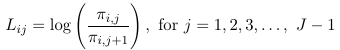
Once one decides what type of logit to use, we construct the logits model with the following identities:

Where Lij are one of the 3 logit types considered above.
These models assume separate intercept for each logit j and the same coefficients for the covariates. The intercept parameters (alpha) are also called cut-point parameters and follow the order of the ordered categorical outcome.
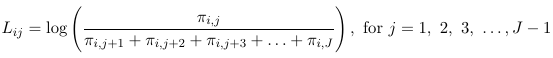
Cumulative Logits Models
A model for the cumulative logits Lij is a model for a binary outcome in which success is defined as any category <= j. Note that the cumulative logits model for a multinomial outcome is not equivalent with J-1 classical logit models. We can also write it as: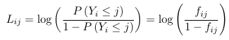
The model also assumes for 2 individuals the relative odds of being at or below a given cut-point (j) on the outcome is independent of the choice of cut-point (j); Meaning separate intercepts for each j of the ordered categorical outcome and the same slope for each predictor. As a consequence of this two individuals i and i' are independent of j:
Because of this, this model is also called the proportional odds model.
The proportional cumulative odds model will estimate a common value for two odds ratios. While the calculations might not always be exactly equal, the estimated values should suggest proportional odds. This can be tested in a logistic model in SAS.
Interpretation
The intercept alpha represents the log odds of having a response <= j when all explanatory variables are 0.
The slope is the increase in logodds of having a response <= j for an individual with characteristics X1 ... Xk than for an individual with characteristics X'1 ... X'k. Particularly it means keeping X2 ... Xk constant each increase of X1 by one unit increases the log odds by beta.
The odds of having a response <= j is:
Each explanatory variable specific odds ratio can be interpreted as the effect of that variable on the ODDS of being in a lower rather than higher category.
Adjacent Categories Logits Models

The same linear combination of predictors applies simultaneously for all J-1 pairs of adjacent response categories. The only thing that varies is the intercept.
Sometimes adjacent logits are defined equivalently as: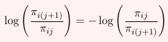
In SAS PROC CATMOD defines the adjacent logits as the former, log(πi(j+1) / πij)
Parameter Interpretation
For two individuals the relative odds of being in category j instead of j+1 is independent of choice of cut-point. Thus for 2 individuals i and i':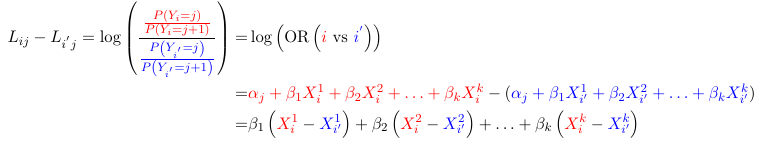
Again, independent of j. That is the ratio of odds of a response j instead of j+1 comparing two groups are the same for every j.
The adjacent odds are exp(![]() ) times higher for an individual with characteristics X1 ... Xk than for an individual with characteristics X'1 ... X'k. Particularly it means keeping X2-Xk constant each increase of X1 by one unit increases the adjacent odds by exp(beta).
) times higher for an individual with characteristics X1 ... Xk than for an individual with characteristics X'1 ... X'k. Particularly it means keeping X2-Xk constant each increase of X1 by one unit increases the adjacent odds by exp(beta).
If we allow the slopes to vary, the proportional odds assumption does not hold.
Continuation Ratio Logits Model
![]()
The same linear logit effect applies simultaneously for all J-1 continuation-ratio logits, the only coefficients that vary are the intercepts.
Let ![]() be the probability of the response in the jth category given that we know the response is >= j.
be the probability of the response in the jth category given that we know the response is >= j.
In other words the continuation-Ratio logits are the ordinary logits of the conditional probabilities of the response being j given that the response is at least j.
Alternatively, some books define the continuation-Ratio logits as:
This is not included in SAS, needs to be programmed.
This model might be more appropriate when ordered categories represent a progression of stages.
Parameter Interpretation
Based on the model for two individuals, the relative odds of being classified in the category j given it is classified in a a >= j category is independent of the choice of cut-point. For two individuals i and i':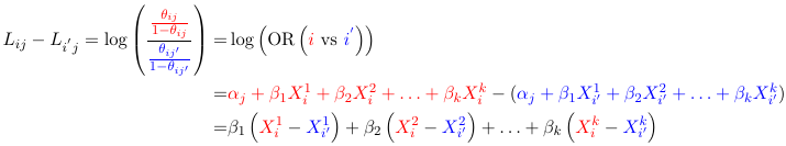
That is the odds of being classified in the jth category given it is classified in a category >= jth comparing two groups is the same for every j.
The continuation ratio odds are exp(![]() ) times higher for an individual with characteristics X1 ... Xk than for an individual with characteristics X'1 ... X'k. Particularly it means keeping X2-Xk constant each increase of X1 by one unit increases the continuation odds by exp(beta).
) times higher for an individual with characteristics X1 ... Xk than for an individual with characteristics X'1 ... X'k. Particularly it means keeping X2-Xk constant each increase of X1 by one unit increases the continuation odds by exp(beta).
SAS Code
SAS is a series of crappy procedures with no coherent structure or consistency.
title2 'Using PROC LOGISTIC  - continuous age linear and quadratic effects';
proc logistic data=contra order=data ;
freq count;
model method=cage agesq/link=glogit ;
output out=aa(where=(_level_ in (1,2) and method in (1,2) and method=_level_)) xbeta=pred;
run;

title2 'Using PROC CATMOD - continuous age linear and quadratic effects';
proc catmod data=contra order=data;
direct cage agesq;
weight count;
model method=cage agesq;
run;

/*Using Genmod*/
title2 'Using PROC GENMOD - continuous age linear and quadratic effects';
proc genmod data=contra;
 class method age;
 model count = method age method*cage method*agesq/dist=p;
run;

axis1 label=('AGE') minor=none order=(1 to 7 by 1) value=(tick=1 '15-19' tick=2 '20-24' tick=3 '25-29' tick=4 '30-34' tick=5 '35-39'
tick=6 '40-44' tick=7 '45-49') ;
axis2 label=(a=90 'Log Generalized Logit (None as reference)') minor=none ;
symbol1 v=circle i=j cv=red ci=blue;
symbol2 v=dot i=j cv=green ci=magenta;
legend1 value=('Observed' 'Predicted') label=('') ;
title1 h=1.2 'Predicted vs. Observed For Method=Sterilization';
proc gplot data=aa;
plot elsn*age pred*age/vaxis=axis2 haxis=axis1 overlay  legend=legend1;;
where method=1;
run;

/* Using SGplot */
ods listing gpath="Z:/Documents/BS853/Spring 2019/Class 6/";
ods graphics / reset width=600px height=400px  imagename="Pred1" imagefmt=gif;
title1 h=1.2 'Predicted vs. Observed For Method=Sterilization';
proc sgplot data=aa cycleattrs;
 yaxis grid label="Log Generalized Logit (None as reference)";
  xaxis grid label="Age";
   series  x=age y=elsn / lineattrs = (pattern=solid thickness=3)
           legendlabel = "Observed Data" name= "elsn";
   scatter x=age y=elsn/ markerattrs=(symbol=circlefilled size=10  color=orange);;
   series  x=age y=pred / lineattrs = (pattern=solid thickness=3)
           legendlabel = "Model" name= "pred";
   scatter x=age y=pred/ markerattrs=(symbol=squarefilled size=10 color=green);
	keylegend "elsn" "pred";
where method=1;
run;

title1 h=1.2 'Predicted vs. Observed For Method=Other';
proc gplot data=aa;
plot elsn*age pred*age/vaxis=axis2 haxis=axis1 overlay  legend=legend1;;
where method=2;
run;

/* Using SGplot */
ods listing gpath="Z:/";
ods graphics / reset width=600px height=400px  imagename="Pred2" imagefmt=gif;
title1 h=1.2 'Predicted vs. Observed For Method=Other';
proc sgplot data=aa cycleattrs;
 yaxis grid label="Log Generalized Logit (None as reference)";
  xaxis grid label="Age";
   series  x=age y=elsn / lineattrs = (pattern=solid thickness=3)
           legendlabel = "Observed Data" name= "elsn";
   scatter x=age y=elsn/ markerattrs=(symbol=circlefilled size=10  color=orange);;
   series  x=age y=pred / lineattrs = (pattern=solid thickness=3)
           legendlabel = "Model" name= "pred";
   scatter x=age y=pred/ markerattrs=(symbol=squarefilled size=10 color=green);
	keylegend "elsn" "pred";
where method=2;
run;


/*Schoolchildren learning style preference and School program*/
/* styles 1=Self,2=Team,3=Class*/
data school;
 do style=1 to 3;
input school program $ count @@;
output;
end;
cards;
1 Regular 10 1 Regular  17 1 Regular  26
1 After    5 1 After    12 1 After    50
2 Regular 21 2 Regular  17 2 Regular  26
2 After   16 2 After    12 2 After    36
3 Regular 15 3 Regular  15 3 Regular  16
3 After   12 3 After    12 3 After    20
run;

title1 'Estimating parameters using contrast statement';
options ls=97 nodate pageno=1;
ods select contrastestimate;
proc logistic data=school order=data;
freq count;
class school program/param=glm;
model style=school program /link=glogit;
contrast 'reg vs. after' program -1 1/estimate=exp;
run;

/*Consider data on association of cumulative incidence of
pneumoconiosis and years working at a coalmine.*/

data ph;
do type=1 to 3;
input age count @@;
output;
end;
cards;
1 218 1 13 1 12
2  71 2 25 2 32
run;

options ls=97 nodate pageno=1;
title1 'Cumulative Logit models - PROC GENMOD';
  proc genmod data=ph order=data descending;
      freq count;  /*<-group data*/
      class age;
      model type = age / dist=multinomial link=cumlogit type3;
      estimate 'LogOR12' age -1 1 / exp;
   run;
title1 'Cumulative Logit models - PROC LOGISTIC';
     proc logistic data=ph order=data descending;
      freq count;
      class age/param=glm;
      model type = age;
     contrast 'LogOR12' age -1 1 / estimate=exp;
   run;

/* Metal Impairement data - Agresti, 1990*/

proc import datafile="Z:\Documents\BS853\Spring 2015\Class 6\impair.xls"
out = mimpair replace;
run;

options ls=97 nodate pageno=1;
title1 'Cumulative Logit models - PROC GENMOD';
  proc genmod data=mimpair rorder=data;
      model level = SES EVENTS/ dist=multinomial link=cumlogit type3;
      estimate 'LogOR12' SES 1  / exp;
   run;

title1 'Cumulative Logit models - PROC LOGISTIC';
    proc logistic data=mimpair order=data ;
     class level;
      model level = SES EVENTS ;
      contrast 'LogOR12' SES 1  / estimate=exp;
   run;
The RESPONSE statement in PROC CATMOD defines the function of the response probabilities (the link function) that we want to model as linear combinations of the predictors. Operations in the RESPONSE statement should be read right to left with the vector of observed response probabilities understood to be the right-most quantity. The rows of the matrices are separated by commas.
The _RESPONSE_ variable is a categorical variable with seperate levels for each of the logits.
/*satisfaction with THR and hospital volume and year of surgery.*/
proc format ;
  value vol 1='High' 0='Low';
run;
data thr;
input  year highvol satisf count;
format highvol vol.;
datalines;
1         0         1        84
1         0         2       231
1         0         3        99
1         1         1       473
1         1         2       493
1         1         3        93
2         0         1       150
2         0         2       347
2         0         3       117
2         1         1       332
2         1         2       387
2         1         3        62
3         0         1       257
3         0         2       889
3         0         3       234
3         1         1       571
3         1         2       793
3         1         3       112
;
run;

options pageno=1 nodate ps=57 ls=91;
title1 'Adjacent Logits models for THR';
proc catmod data=thr;
  weight count;
  response ALOGIT;
  model satisf= _response_ highvol year;
run;
quit;


/* let the effect of year vary with the cutpoint*/
title1 'Adjacent Logits models for THR - with coefficents dependent on the level of satisfcation';
proc catmod data=thr ;
  weight count;
  response ALOGIT;
  model satisf= _response_ highvol _response_|year;
run;
quit;


/* number of hip fractures by race age and BMI */
/* n=0 then no hip fractures, n=1 then 1 hip fractures, n=2 then more than 1 hip fractures */
data nhf;
do n=0 to 2;
input race $ age $ bmi count @@;
output;
end;
cards;
white	<=80 	1	39	white	<=80 	1	29	white	<=80 	1	8
white	<=80	2	4	white	<=80	2	8	white	<=80	2	1
white	<=80	3	11	white	<=80	3	9	white	<=80	3	6
white	<=80	4	48	white	<=80	4	17	white	<=80	4	8
white	>80 	1	231	white	>80 	1	115	white	>80 	1	51
white	>80	    2	17	white	>80	    2	21	white	>80	    2	13
white	>80	    3	18	white	>80	    3	28	white	>80	    3	45
white	>80	    4	197	white	>80	    4	111	white	>80	    4	35
black	<=80 	1	19	black	<=80 	1	40	black	<=80 	1	19
black	<=80	2	5	black	<=80	2	17	black	<=80	2	7
black	<=80	3	2	black	<=80	3	14	black	<=80	3	3
black	<=80	4	49	black	<=80	4	79	black	<=80	4	24
black	>80 	1	110	black	>80 	1	133	black	>80 	1	103
black	>80	    2	18	black	>80	    2	38	black	>80	    2	25
black	>80	    3	11	black	>80	    3	25	black	>80	    3	18
black	>80	    4	178	black	>80	    4	206	black	>80	    4	81
;
run;
options pageno=1 nodate ps=57 ls=91;
/* continuation ratio logits models*/
 title1 'Continuation-ratio Logits models for NHF using the response statement';
proc catmod data=nhf;
     weight count;
     response * 1 -1 0  0,
                0  0 1 -1  log  * 1 0 0,
                                  0 1 1,
                                  0 1 0,
                                  0 0 1;  /* p1
                                             p2
                                             p3  */
     model n=_response_ age bmi|race/  predict;
     run;
     quit;

	 /* Use second way to defining continuation ration logits */
title1 'Continuation-ratio Logits models for NHF using the response statement(2)';
  proc catmod data=nhf;
     weight count;
     response * -1 1  0 0,
                 0 0 -1 1  log  * 1 0 0,
                                  0 1 0,
                                  1 1 0,
                                  0 0 1;
     model n=_response_ age bmi|race/ prob predict;
     run;
     quit;

/* let the coefficients depend on the number of hip fracturs */
 title2 'Coefficients dependent on the number of HF';
proc catmod data=nhf;
     weight count;
     response * 1 -1 0 0,
                0 0 1 -1  log  * 1 0 0,
                                 0 1 1,
                                 0 1 0,
                                 0 0 1;

     model n=_response_|bmi _response_|age _response_|race  bmi|race/ freq;
     run;
     quit;

title1 'Adjacent Logits models for THR using the response statement';
proc catmod data=thr;
  weight count;
 response * -1  1 0,
             0 -1 1  log  * 1 0 0,
                            0 1 0,
                            0 0 1;  /* p1
                                       p2
                                       p3  */
  model satisf= _response_ highvol year;
run;
quit;

title1 'cumulative Logits models for THR using the response statement';
proc catmod data=thr;
  weight count;
 response *  1 -1 0  0,
             0  0 1 -1  log  * 1 0 0,
                               0 1 1,
                               1 1 0,
                               0 0 1;  /* p1
                                       p2
                                       p3  */
  model satisf= _response_ highvol year;
run;
quit;
title1 'cumulative Logits models for THR using Proc Logistic ';
proc logistic data=THR;
  class highvol year;
  model satisf= highvol year;
  freq count;
run;

/********************************************************************************/
/***               Overdispersion in binomial models                          ***/
/********************************************************************************/
DATA aggregate;
  INPUT pot total yes cultivar soil @@;
cards;
 1 16  8 0 0   2 51 26 0 0
 5 36  9 0 0   6 81 23 1 0
 9 28  8 1 0  10 62 23 1 0
13 41 22 0 1  14 12  3 0 1
17 30 15 1 1  18 51 32 1 1
 3 45 23 0 0   4 39 10 0 0
 7 30 10 1 0   8 39 17 1 0
11 51 32 0 1  12 72 55 0 1
15 13 10 0 1  16 79 46 1 1
19 74 53 1 1  20 56 12 1 1
;
run;


/* no scale - aggregated data'*/
options pageno=1 nodate ps=57 ls=91;
title1 ' No Scale ';
proc genmod data=aggregate;
model yes/total = cultivar|soil/type3 dist=binomial ;
run;

/*  scale - aggregated data'*/
/* Model 2 */
title1 ' Scale parameter estimated by the scaled dispersion ';
proc genmod data=aggregate;
model yes/total = cultivar|soil/type3 dist=binomial dscale ;
run;
GLM for Count Data
Generalized linear models for count data are regression techniques available for modeling outcomes describing a type of discrete data where the occurrence might be relatively rare. A common distribution for such a random variable is Poisson.
The probability that a variable Y with a Poisson distribution is equal to a count value
$${ P(Y = y) = {{\lambda^y e^{-\lambda}} \over {y!}}} y = 0, 1, 2, ..., \infty $$
where λ is the average count called the rate
The Poisson distribution has a mean which is equal to the variance:
E(Y) = Var(Y) = \(\lambda\)
The mean number of events is the rate of incidence multiplied by time passed
Because of this assumption, the Poisson distribution also has the following properties:
- If Y_1 ~ Poisson(λ_1) and Y_2 ~ Poisson(λ_2) where Y_1 and Y_2 are the number of subjects in groups 1 and 2, then Y_1 + Y_2 ~ Poisson(λ_1 + λ_2)
- This generalizes to the situation of n groups as: Assuming n independent counts of Y_i are measured, if each Y_i has the same expected number of events λ then Y_1 + Y_2 + ... + Y_n ~ Poisson(nλ). In this situation λ is interpretable as the average number of events per group.
Poisson Regression as a GLM
To specify a generalized linear model we need (1) the distribution of outcome, (2) the link function, and (3) the variance function. For Poisson regression these are (1) Poisson, (2) Log, and (3) identity.
Let's consider a binomial example from a previous class where:
$$ Y_{ij} \approx Binomial(N_{ij}, λ_{ij}) $$
Given a variable Y ~ Binomial(n, p), where n is number of experiments and p the probability of success, this binomial distribution can be approximated well by the Poisson distribution with mean n*p.
So from that we can assume the distribution of Y also follows:
$$ Y_{ij} \approx Poisson(N_{ij} λ_{ij}) $$
and thus
$$ log(E(Y_{ij})) = log(N_{ij}) + log(\lambda_{ij}) $$
Since log(N_ij) is calculated from the data, we will proceed by modeling log(λ_ij) as a linear combination of the predictors:
$$ log{λ_{ij} } = μ + β_1X_{ij}^1 + β_2 X_{ij}^2 + . . . + β_k X_{ij}^k $$
The natural log is attractive as a link function for several reasons:
- The log link maps relative rates into additive effects
- With this link, parameters are readily interpretable as rate ratios, these ratios are called relative risks (risk ratios)
- The log link transforms positive values into the whole real link.
This the Poisson regression models extend the loglinear models; loglinear models are instances of Poisson regression.
Modeling Details
With the assumption
$$ E(Y_i) = N_i*λ_i $$
then using a log link we have:
$$ log(E(Y_{i})) = log(N_{i}) + log(\lambda_{i}) $$
Assuming we have a set of k predictors X1, X2, ..., Xk (continuous and/or ordinal and/or nominal), in Poisson regression one the linear predictors can be represented as:
$$ log{λ_i} = μ + β_1X_{i}^1 + β_2 X_{i}^2 + . . . + β_k X_{i}^k $$
We can represent the expected value as: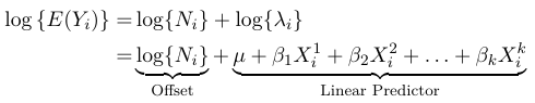
Where the term log(N_i) is called the offset. The offfset allows us to consider groups of different sizes in the model, but carries little value in terms of outcome.
In SAS we can use GENMOD to specify the Poisson distribution and an optional offset, but we must calculate the value ourselves.
proc genmod data = claims ;
class district car age ;
model C = district car age / offset = logN dist = poisson link = log obstats ;
estimate ’ district 1 vs . 4 ’ district 1 0 0 -1/ exp ;
run ;
In the results, the distribution of the chi-squared residuals (or deviance residuals) can be approximated by standard normal distribution. When the number of cells is large this assumption can be checked via a normal quantile plot, such as PROC UNIVARIATE; A linear pattern is evidence of a good fit.
Interpretation of Parameters
Interpretation is much the same as in a binomial model, we compare the rate of incidence in the reference group to that of the other groups:
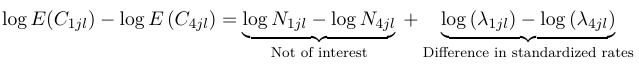
The most common use of a Poisson regression is in the analysis of time-to-event or survival. In cohort studies, the analysis of data usually involves estimation of disease during a defined period of observation; In this case the denominator of such a rate is measured in years of observation per person (person-years).
Over-dispersion in Poisson Regression
Over-dispersion occurs when the variance of the response exceeds the mean (nominal variance in Poisson); That is:
$$ var(Y) > E(Y) = n \pi (1 - \pi) $$; Where n is the number of trials and π is the probability of success
This can be the result of several phenomena:
- When the response is a random sum of independent variables, that is Y = R_1 + R_2 + ... + R_k where k is distributed as Poisson independent of R_i's
- When Y ~ Poisson(L), where L is random (this appears when there is inter-subject variability). The classical assumption is that L ~ Gamma(α, μ)
- When missing important covariates
- When the total population (N) is random rather than fixed
Regardless of the source of over-dispersion, methods that take the over-dispersion into account should not be used. Not taking into account the over-dispersion results in many false positive test results, as without taking into account the over-dispersion the estimates for the variability of the coefficients underestimates the scale of w.
We can use a generic method to model the over-dispersion by modifying the variance function from the identity function g(λ) = λ to g(λ) = w2λ. w is called the scale or over-dispersion parameter.
An estimator for w is:
$$ w^2 = {X^2 \over {n-p}}= { \sum_i {(n_i - \hat m_i)^2 \over \hat m_i} \over {n-p} }$$
Where p is the number of parameters and n is the number of observations. If w > 1 we say there is over-dispersion. A similar estimate might be obtained by replacing the Pearson chi-square statistic with the Deviance statistic. One can test for over-dispersion using the Negative Binomial Generalized Linear Model.
Testing for Over-Dispersion in Poisson - Negative Binomial Regression
Scaled deviance and scaled Pearson Chi-Squared can be used to detect over-dispersion or under-dispersion in the Poisson regression. We can test for over-dispersion by comparing deviances from a generalized linear model based on Poisson distribution assumption for the outcomes with log link and offset and a generalized linear model based on the negative binomial distribution assumption for the outcome with a log link and offset.
For a negative binomial distribution: var(Y) = E(Y) + k{E(Y)}2
Where k >= 0 (the negative binomial likelihood reduces to Poisson when k = 0)
In testing over-dispersion in a Poisson regression the hypotheses are: H0: k=0 vs Ha: k > 0
The negative binomial regression can be fit in SAS as the Poisson regression, with the change that in the dist option we specify 'NB'.
To carry out the test:
- Run a Poisson Regression
- Run the Negative Binomial
- Subtract the log-likelihood values from teh negative binomial regression and Poisson regression and multiply by 2 to obtain the test statistic
O = 2 * (LL(Negative Binomial) - LL(Poisson)) - If the test significance level is α, compare it against a critical value from a Chi-Square distributino with one degree of freedom and level 2α
title2 ’ Using GENMOD - Poisson Regression ’;
ods select Modelfit ;
proc genmod data = incidence ;
class age race ;
model cases = age race / dist = poisson link = log offset = logT ;
run ;

title2 ’ Using GENMOD - Negative Binomial Regression ’;
proc genmod data = incidence ;
class age race ;
model cases = age race / dist = NB link = log offset = logT ;
run ;
Note: Under-dispersion cannot be tested with this method.
Zero-Inflated Poisson
Zero-Inflated Poisson (ZIP) and Negative-Binomial Models deal with situations where there is an added number of instances of data with a count of 0. Zero-inflated models have become fairly popular and have been implemented in many statistical packages.
The ZIP model is one way to allow for over-dispersion with Poisson data. The model assumes that the data values come from a mixture of two top distributions: one set of counts from a standard Poisson distribution, and the other that generates zero counts with probability 1. The value 0 could come from either of the two distributions. A Bernoulli generalized linear model can be used to predict which group an individual belongs to: the one in which the values come from the distribution that only generates 0 counts or from one that follows a Poisson distribution.
The ZIP can be thought of as a latent class model. The assumption being that there exists a Bernoulli (unobserved) variable Z that indicates whether the count comes from the certain 0 distribution or from a Poisson distribution. First remember that for a Poisson variable Y:
$${ P(Y = y) = {{\lambda^y e^{-\lambda}} \over {y!}}} $$
and thus:
$$ P(Y = 0) = {{ e^{-\lambda}}} $$
For an individual i, Zi = 1 then the count will be 0, while if Zi = 0 then the count comes from the Poisson distribution. If P(Zi = 1) = \(\pi_i\) then:
$$ P(Y_i = 0 | X_i) = \pi_i + (1 - \pi_i) P(0|X_i) = \pi_i + (1 - \pi_i) e^{ -\lambda_i } $$
$$ P(Y_i = y | X_i) = (1 - \pi_i)P(y | X_i) =(1 - \pi_i) {{\lambda^y e^{-\lambda}} \over {y!}} $$ for y > 0
The mean of this variable:
$$ E(Y_i | X_i) = (0 * \pi_i) + \lambda_i (1 - \pi_i) = \lambda_i (1-\pi_i) $$
The variance is:
$$ Var(Y_i | X_i) = \lambda_i (1 - \pi_i) (1 + \lambda_i \pi_i) $$
Noting that Var(Yi | Xi) > E(Yi | Xi), so the variance is larger than a Poisson variance.
One can then proceed by modeling both the parameter π (mixture probability) and the parameter λ (the mean of the Poisson count) as a function of the covariates by first transforming these parameter values using link functions.
Often a logit link is used for the π and a log link for λ. In other words the model assumes:
- For the π parameter assume the identity
\( log( {\pi_i \over {( 1 - \pi_i) }} ) = \gamma X_i \) - For the λ parameter assume the identity
log(λi) = β Zi
The covariates in the model for π can be different or the same as the covariates in the model for λs. A Zero-Inflated negative binomial (ZINB) can be defined similarly.
In cases with excess 0's the ZIP model usually fits better than a Poisson generalized linear model. Often, a negative Binomial model fits well with data that has excess of zeros. The ZINB model fits better than a conventional Negative Binomial model regression model if the data present with both over-dispersion and excess of zeros.
title1 ’ Zero Inflated Poisson Regression ( Model 7) ’;
proc genmod data = absences ;
class C S A L / param = ref ;
model days = C | A | S | L @2 / dist = zip ;
zeromodel C S / link = logit ;
run ;
The interpretation of parameters for the above model is complex because of the presence of three two-way interactions, but the steps involved would follow the interpretation in the Poisson regression model.
Gamma Regression
Consider a continuous dependent variable that is positive-valued, such as a length of a hospital stay, time waiting or the cost of a bill. This type of data is continuous in nature and oftentimes skewed and a normal approximation does not hold.
The type of data above presents a constant Coefficient of Variation (CV), that is:
$$ \sqrt{var(Y_i)} \over E(Y_i) = \sigma $$
The identity induces a quadratic variance function:
$$ var(Y_i) = \sigma^2E(Y_i)^2 $$
To model such data a number of approaches proposed in the literature have proved useful, including Log-Normal models and Gamma Regression models
- Log Normal models - the log transformation followed by a classical linear model is fairly successful in modeling this type of data. This approximation works best when the scale parameter (sigma) is small. Indeed, the log transformed model has approximately constant variance:
$$ log(Y) \approx log(\mu) + (Y - \mu) {{\delta log(y)} \over {\delta y}}(\mu) = log(\mu) + {{Y - \mu} \over \mu} $$
$$ Var(log(Y)) \approx {Var(Y) \over \mu^2 } = {{\sigma^2\mu^2} \over \mu^2 }= \sigma^2 $$ - Gamma Regression - the Gamma regression keeps the outcome on the original scale. If one wants to work on the original scale the framework of the generalized linear model proves very fruitful.
Gamma Distributions
The Gamma family is a very flexible family of distributions with support on the positive axis. The family is indexed by two parameters. One way to parameterize which is used in SAS and focused on in this lecture is called the mean parameterization.
A variable is said to follow the Gamma distribution if the density has the form:
$$ f_Y(y) = {1 \over {\Gamma (v)y} }({{yv \over \mu}})^v exp(-{{yv} \over \mu}), 0 < y < \infty $$
where
$$ \Gamma(v) = \int_0^\infty x^{v-1}exp(-x)dx $$
The mean and variance of a Gamma distributed variable are:
$$ E(Y) = \mu $$
$$ var(Y) = {\mu^2 \over v } = \sigma^2\mu^2, \sigma^2 = {1 \over v} $$
The parameter v is called the scale parameter, and \( v / \mu \) is called the rate parameter. The inverse of the scale parameter (\(\sigma^2\)) is called the dispersion parameter.
Properties of the Gamma Distribution
- The shape of the density is controlled by v
- Regardless of the value of v the densities are skewed to the right
- When v < 1 the Gamma distribution is exponentially shaped and asymptotic to both vertical and horizontal axes
- A Gamma distribution with scale parameter v = 1 and mean parameter μ is the same as an exponential distribution with mean parameter μ. In SAS we can actually test whether v = 1
- When v > 1 the Gamma distribution assumes a unimodal but skewed shape. The skewedness reduces as the value of v increases. As v tends to ∞ the Gamma distribution begins to resemble a normal distribution.
- The chi-sqaure distribution is a special case of the Gamma. A chi-sqaure distribution with n degrees of freedom is the same as a Gamma with \( v = {n \over 2} \) and \( \mu = n \)
- The Gamma is a flexible life distribution model that may offer a good fit to some sets of failure data. However, it is not widely used as a life distribution model for common failure mechanisms.
- The Gamma does arise naturally as the time-to-first failure distribution for a parellel system with components having lifetimes distributed exponentially. If there are components in the system and all components have exponential lifetimes with mean \(\gamma\), then the total lifetime has Gamma distribution v = n and \(\mu = n\gamma \)
- The Gamma distribution is widely used in engineering, science and business.
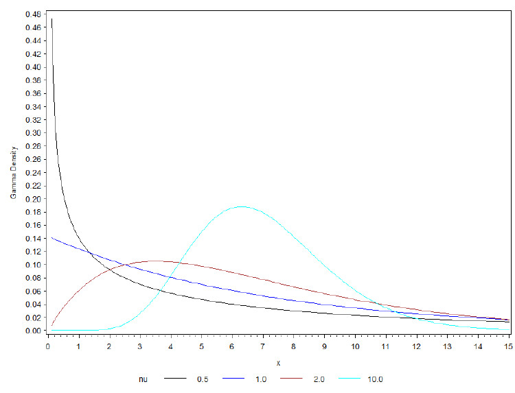
The above is an example of different shapes of the Gamma distribution with different values of v and μ = 7
Gamma as a Generalized Linear Model
As with all Generalized Linear Models, to specify the Gamma regression as a GLM we need to specify the link and variance function besides the distribution of the response.
- Variance function is V(μ) = a*μ2
- The most commonly used link function are the Log (g(μ) = log(μ)) and inverse (g(μ) = 1 / μ). The default in SAS is inverse
- With inverse link, a change in the coefficients will induce an opposite change in the expected value of the response, with log link the opposite is true
- The inverse link does not map the expected value μ into the whole real line; therefore we have to be careful when we interpret parameters
Interpretation
Assume we have a dichotomous exposure X (1 = yes, 0 = no). If the log link is used we can describe the regression as:
$$ log(\mu(X)) = \alpha + \beta*X $$
The coefficient β is interpreted in terms of Mean Ratio (MR)
$$ MR = {{exp(\alpha + \beta)} \over {exp(\alpha)}} $$
The increase in logarithm of means for one unit increase in X.
With an inverse link a change in the coefficients will induce an opposite change in the expected value of the response.
$$ {1 \over {\mu(X)}} = \alpha + \beta*X $$
The coefficient β is interpreted in terms of Inverse Mean Difference (IMD)
$$ IMD = {{1 \over \mu_{X=1}} - {1 \over \mu_{X=0}}} = \alpha + \beta - \alpha = \beta $$
One unit increase in X causes and increase of β in the inverse of means.
With log link the interpretation of the parameters is similar to the logit models; however the odds are replaced by the means, and the OR is replaced with mean ratios:
$$ log( {\mu_i \over \mu_{i'}}) = \beta(X^1_i - X^1_{i'})$$
The expected response is multiplied by exp(β) for each unit change in X1
With inverse power metric a change in the coefficients will induce an opposite change:
$$ {1 \over \mu_{i}} - {1 \over \mu_{i'}} = \beta(X^1_i - X^1_{i'})$$
The inverse of the expected response changes by β for each unit change in X. If β > 0 then the mean decreases with an increase in X, while if β < 0 then hte mean increases with an increase in X.
Measuring Goodness of Fit
The log-likelihood for a given model M: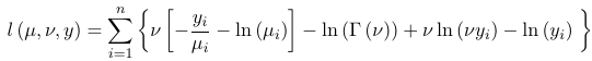
The log-likelihood for a saturated model: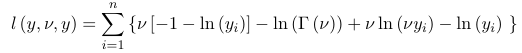
Thus the deviance is:
In Gamma regression the scaled deviance and the scaled Pearson chi-square are measures of goodness of fit statistics. For the Gamma distribution \(\sigma^2 = {1 \over v} \). If v is a known priori for a model M that has p parameters and n observations, the scaled deviance and scaled Pearson chi-square are:
$$ {D \over \sigma^2 } $$ and $$ {{X^2 \over \sigma^2} \approx \chi^2_{n-p'}}$$
That is reject the model if:
$$ {D \over \sigma^2 } > \chi^2_{n-p, 1-\alpha} $$
Where σ is estimated from the data. Thus to compare two nested models, with p and 1 parameters:
$$ {{D_{M_2} - D_{M_1}} \over \sigma^2} \approx \chi^2_{p-1} $$
These estimates can be very unstable; however, one reasonable approach is to estimate it in the largest model we are willing to consider then use that estimate in model selection.
Estimating the Dispersion Parameter
For a Gamma distributed variable Z, with Mean = E(Z) = μ and Variance = Var(Z) = 𝜎2μ2, with a response Yi for subject i we can estimate variance as:
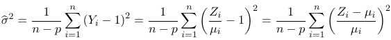
For a normal linear regression a similar result holds. The scale parameter in PROC GENMOD is the standard deviation.
Exploratory Data Analysis
To check the assumptions of a Gamma regression and to help choose an appropriate function form and link function you can plot the predictors X vs log(E(Y)) and 1/E(Y). The more appropriate link would appear linear.
With ordinal predictors you would compute the raw means of the response at each level of the predictor while for continuous outcomes you can aggregate values of predictors and treatment as ordinal.
SAS Code
/*****************************************************************/
/*** Gamma Model - Log normal                           ***/
/*****************************************************************/
title1 'Gamma regression - Saturated model';
title3 'Inverse Link';
proc genmod data=claims;
class policyholderage cargroup ageofcar ;
model lcost=policyholderage|cargroup|ageofcar @2	/dist=normal ;
weight number;
run;

/*****************************************************************/
/*** Gamma Model - Log Link                            ***/
/*****************************************************************/
title1 ' Gamma regression - Saturated model';
title3 'Log Link';
proc genmod data=claims;
class policyholderage cargroup ageofcar ;
model cost=policyholderage|cargroup|ageofcar 	/dist=gamma link=log ;
weight number;
run;
Survival - Time to Failure
Analysis of survival data is more complex than than other methods we've seen so far; We can't just take the mean survival time a a confidence interval to predict when the last patient will die. Also, survival times are unlikely to follow a Normal distribution, so simple regression techniques are not applicable.
Censoring
Censoring of data can happen in a number of ways:
- Some subjects still have not experienced the event of interest by the end of the study. Most studies have a recruitment period followed by a pure follow-up period. Patients who are enrolled earlier have a higher chance of experiencing the event.
- Some participants drop out early, either due to dropping out or another event unrelated to the study.
In either case, you know that the subject has participated in a study to a certain time without witnessing the event, but have no information thereafter. Such incomplete information is said to be right censored. Note that we censor the data, not the subject. Throughout this lecture we will assume independent censoring - the participants remaining in the study are representative of the target population.
Methods of Analyzing Survival
Let's consider a dataset of rats testing a new cancer treatment.
Approach 1: Test for Difference in Outcome After a Set Time (Wrong)
We could pick a set number of days and consider the number of rats in each group. We can use a chi-square test to determine if the outcome between the two groups is the same. A 95% confidence interval for the population could also be determined.
The problem with this approach is it disregards exact death times and ignored censored observations before the cutpoint. Comparing survival at a single point in time is not informative, the results could change significantly at a different cutpoint.
Approach 2: Comparing Incidence Rates
Estimates can be obtained for the incidence rates, by taking the number of deaths and the population follow-up time in each group. We would expect the proportion of cases will be the same under the null hypothesis. The estimate of the rates can also be obtained by using a Poisson regression.
SAS Script
data one ;
input Group C Time ;
LogT = log ( Time ) ;
cards ;
1 17 4095
2 19 5023
run ;

proc genmod data = one ;
class Group ;
model C = Group / dist = poisson offset = LogT ;
estimate ’ Group 1 ’ Intercept 1 Group 1 0/ exp ;
estimate ’ Group 2 ’ Intercept 1 Group 0 1/ exp ;
Estimate ’ Group 2 vs 1 ’ Group -1 1/ exp ;
Run ;
Approach 3: Consider Follow-Up Time to be a Stratifying Variable
Compare rates between groups in the first 200 days, days 201-250 and 251-300. Dropouts/censoring occur at the end of each interval.
We could make a 2x2 table for each strata and use the Cochran - Mantel - Haenszel test statistic for Group 1 vs Group 2 survival.
/* Comparing survival using CMH test and 3 time strata */
data RCMH ;
do group =1 to 2;
Do time =1 to 3;
input yes no @@ ;
output ;
end ;
end ;
cards ;
6 13 9 4 1 1
4 17 9 8 5 2
run ;

proc sort data = RCMH ;
by group time ;
run ;

proc transpose data = RCMH out = RCMH2 prefix = count name = died ;
by group time ;
run ;

/* Comparing survival using CMH test and 3 time strata */
title1 ’ Comparing survival using CMH test and 3 time strata ’;
options pageno =1 ps =57 ls =91 center nodate ;
proc freq data = RCMH2 order = data ;
table time * group * died / cmh chisq relrisk ;
weight count1 ;
run ;
Approach 4: Log-Rank Test (Best)
Taking smaller intervals gives a more refined test. If the intervals are chosen based on the event times, that is each interval starts and ends with an event, the resulting test is the log-rank test.
Here the censored obesrvations are followed through the last interval they complete. In the data, to fully specify the each subject we must provide (1) a time of follow-up and (2) an indicator of whether censorship or the terminating event occurs at that time.
This can be performed by hand; however, it can get computationally intensive. The Log-Rank test can be directly obtained from SAS from PROC LIFETEST; the risk variable should be specified in the STRATA statement.
SAS Script
data ratc ;
input group day censor @@ ;
logt = log ( day ) ;
cards ;
1 143 0 1 220 0 2 156 0 2 239 0
1 164 0 1 227 0 2 163 0 2 240 0
1 188 0 1 230 0 2 198 0 2 261 0
1 188 0 1 234 0 2 205 0 2 280 0
1 190 0 1 246 0 2 232 0 2 280 0
1 192 0 1 265 0 2 232 0 2 296 0
1 206 0 1 304 0 2 233 0 2 296 0
1 209 0 1 216 1 2 233 0 2 323 0
1 213 0 1 244 1 2 233 0 2 204 1
1 216 0 2 142 0 2 233 0 2 344 1
run ;

title1 ’ Using Log - Rank test ’;
options pageno =1 ps =57 ls =91 centerPROC LIFETEST data = ratc notable ;
TIME day * censor (1) ;
STRATA group ;
run ;
Note that the censoring variable contains the label associated with observation being censored in parentheses.
Survival Function
Denote T as the time to event for an individual. The survival function (denoted by S(t)) is defined as:
$$ S(t) = P(T > t), 0 \leq t < \infty $$
In other words, S(t) is the probability the individual survives beyond time t.
The Cumulative Distribution Function (CDF) of the random variable T is defined as F(t) = P(T <= t) and is related to the survival function through: F(t) = 1 - S(t)
Suppose T is a continuous random variable. In this case, the hazard function λ(t), is defined as the instantaneous rate of failure at T = t conditional on surviving beyond T = t. Note the hazard is NOT a probability.
More precisely, since the probability of an event in the interval (t, t + δ) given the event has not occurred up to time t, is P(t < T <= t + δ|T > t), the hazard is obtained by dividing the probability by the length of the interval and defining a limit. In other words:
$$ \lambda(t) = \lim_{\delta \to 0+} {{P(t < T \leq t + \delta | T > t)} \over {\delta}} $$
Some simplification reduces this to F'(t) / S(t) or f(t) / S(t), where F'(t) or f(t) is the probability density function (the derivative of F(t)). From linking the survival function to the cumulative distribution function we know F'(t) = -S'(t), so we can further reduce the hazard to:
$$ \lambda(t) = d log S(t) / dt $$
and integrating both sides with respect to t and using the fact that S(0) = 1:
$$ S(t) = exp( - \int_0^t \lambda(s) ds) $$
Which gives us the cumulative hazard function:
$$ A(t) = \int_0^t \lambda (s) ds $$
Which we can simplify again to get the density function as a product of the hazard function:
$$ f(t) = \lambda(t) exp(-\int_0^t \lambda(s) ds) $$
All three parameters (survival, cumulative hazard and density) are related. If one parameter is specified the other 2 can be derived.
Life Table Estimates
Life tables are used to describe pattern of survival in populations. These methods can be applied to the study of any time to event endpoint.
The life table method requires a pre-specification of a set of intervals that span the follow-up time. The life-tables are computed by counting the numbers of censored and uncensored observations that fall into each of the time intervals.
The conditional probability of an event in the interval Ii = [ti,ti+1) given that the event did not occur up to time ti that is P(T ∈ Ii | T > ti) is estimated by:
$$ p_i = r_i / m_i $$
where r is the number of events in the interval, I and m = n - c/2 are called the effective sample size, equal to the number of patients at risk (n) in the interval m minus half the number of censored observations (c) in the interval I. This is because the assumption of the life-table is that any censored observation with an interval is treated as if it were censored at the midpoint of the interval. So, since the censored observations are at risk for only half the interval they count for only half in figuring out the number at risk.
The estimated variance of pi and its estimated standard error is:
$$ var(p_i) = {{ p_i (1 - p_i) } \over m_i} $$
The product limit estimate of the survival function at ti is obtained by piecing together the conditional probabilities pi estimated above.
$$ \hat S (t_0) = 1 $$
$$ \hat S (t_i) = P(T > t_i) = P(T < t_i | T > t_{i-1})P(T > t_{i-1}) = (1 - p_{i - 1})\hat S(t_{i-1}) =(1 - p_{i - 1})(1 - p_{i - 2})... (1 - p_{1})(1 - p_{0}) $$
$$ Var(\hat S(t_0)) = 0 $$ $$ Var(\hat S(t_i)) = \hat S(t_i)^2 \sum_{j=1}^{i-1} {p_j \over {m_j (1-p_j}}$$
The Life-Table function estimates are piecewise constant functions with estimates at the midpoint at each interval. Calculated as:
$$ h(t_{im}) = {r_i \over {w_i(n_i - {c_i \over 2} - {r_i \over 2})}} $$
Where for the ith interval, t is the midpoint, r is the number of events, w is the width of the interval and n is the number still at risk at the beginning of the interval, and c is the number of censored observations within the interval. The estimate assumes the events occur at the middle of the interval.
title ’ Angina Pectoris in Framingham study ’;
data anginaf ;
input censor time sex freq @@ ;
years =1.5+3* time ;
cards ;
0 0 1 33 0 0 2 35
0 1 1 64 0 1 2 50
0 2 1 59 0 2 2 63
0 3 1 76 0 3 2 85
0 4 1 83 0 4 2 85
0 5 1 99 0 5 2 91
0 6 1 110 0 6 2 91
0 7 1 105 0 7 2 87
0 8 1 932 0 8 2 1561
1 0 1 139 1 0 2 82
1 1 1 34 1 1 2 31
1 2 1 36 1 2 2 35
1 3 1 30 1 3 2 42
1 4 1 37 1 4 2 39
1 5 1 39 1 5 2 37
1 6 1 31 1 6 2 34
1 7 1 37 1 7 2 42
1 8 1 0 1 8 2 0
run ;

title ’ Angina Pectoris in Framingham study ’;
proc lifetest data = anginaf method = lt intervals=(1.5 to 25.5 by 3);
time Years * Censor (0) ;
freq Freq ;
strata sex ;
run ;
Kaplan-Meier Estimate
The Kaplan-Meier estimate of the life table estimate is a non-parametric estimate of S(t) with intervals being create by failure times.
Suppose we have order failure time 0 < t1 , t2 ... < tm, so that for any tk < t < tk+1. The Kaplan-Meier estimate is obtained by estimating each term separately and then multiplying the estimates. Corresponding to each tk let nk be the number "at risk" just prior to time tk and dk be the number of deaths at time tk.
An estimate of P(tk < t < tk+1 | T > tk-1) is the proportion of events in the interval (dk) among the subjects still at risk at the beginning of the interval which is nk. Thus the estimate of the proportion of deaths is \( d_k \over n_k \)
Multiply all the estimates together to get the Kaplan-Meier estimator (or the product-limit estimator) of S(t):
$$ \hat S(t) = \prod_{j | t_j < t} {{n_j - d_j}\over n_j} $$
The survival functions in each group are estimated using the Kaplan-Meier method. Often the Log transformed or Log(-Log()) transformed survival functions. If the curves are parallel between groups then proportional hazards can be employed (discussed more later).
The Wilcoxon test is another method for comparing survival curves. It is similar to Log-Rank but places more weight on early survival times while Log-Rank places more weight on later survival times.
Accelerated Failure Time Models
Let's assume a time to event outcome with 3 predictors. We want to study the association between these predictors and the distribution of a time to event outcome. In Accelerated Failure Time Models (AFTM) the response is chosen to be the Log of time to event, then we model it as a linear combination of the predictors and an error term which is scaled by a parameter sigma with a known distribution:
This resembles the classical linear regression model but we want to be able to accommodate censored data.
1. First assume the scale sigma = 1 and beta_0 = 0. Then:
Where Ti0 is a baseline time to event for X1 = X3 = X3 = 0 whose distribution is assumed known. Thus the survival times distributions for individuals with covariate values Xi1 = xi1, Xi2 = xi2, and Xi3 = xi3, is changed by a scale factor from a baseline distribution of T0.
Using this model, the survival distribution is: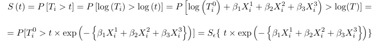
2. If we allow for a nonzero intercept and a scale parameter, then the above becomes: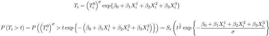
where S is the survival function of the survival time T0
Constructing the Likelihood (Assuming Right Censoring)
The time to event observations t1, t2 ... tn are assumed independent, and this the likelihood is a product of the contribution from each observation. There are two types of observations (a) censored observations and (b) event times.
a) If the observation is a censored time the the contribution is P(T > ti) = S(ti)
b) If the observation is an event time, the the contribution is f(ti) where f is the density
Thus the likelihood: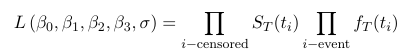
which is then maximized over theta to obtain point estimates for the betas and sigma. This is too hard to do by hand so SAS has PROC LIFEREG to fit this type of model. It assumes right censoring but other types of censoring can be accommodated.
GLM for Correlated Data
So far the models we've covered assume independence between observations collected on separate individuals. When observation are correlated models that incorporate the existing correlation in the data should be employed. There are many approaches are proposed but here we focus on Generalized Estimating Equations (GEE) and Mixed Effects Generalized Linear Models.
Generalized Estimating Equations Methods
For classical generalized linear model we assume only one observation was collected per subject with a set of predictors.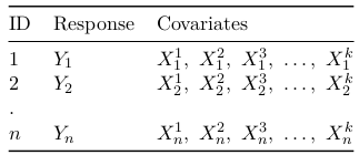
The most common type of correlated data is longitudinal, collected on the same subjects over time. For data with 3 time points: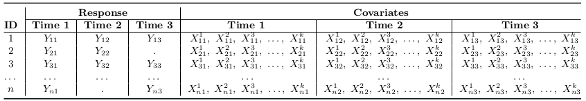
Other examples of correlated data are: Data collected from different locations on the same subject or collected on different subjects which are related.
In SAS the function to estimate GEE models is PROC GENMOD. For normal models it can be fit in other procedures, such as PROC MIXED. Using PROC GENMOD the data must be inputted in long form (multiple observations per subject):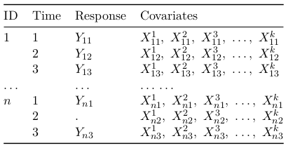
Now we could analyze the data by observing the counts out the outcome while ignoring the correlation between subjects, or simply observe the linear correlation between outcome and time, but in general ignoring the dependency of the observations will in general overestimate the standard errors of the time-dependent predictors since we haven't accounted for within-subject variability.
The influence of correlation on statistical inference can be observed by inspecting its influence on the sample size for a design that collects data repeatedly over time. In comparing 2 groups in terms of means on a measured outcome Yij where i is subjects and j is group, and in each group there are m subjects and within each group there are n repeated observations. Further assuming that Var(Yij) = σ2 and that within each group Cor(Yij, Yhj) = ρ where i != h. Then the sample size needed to detect a difference in means of outcome, d = μ1 + μ2 = E(Yi1) - E(Yi2) with power P = 1 - Q and type I error (α) is:
$$ m = {{2(z\alpha + zQ)^2\sigma^2(1 + (n - 1)\rho)} \over {nd^2}} = {{2(z\alpha + zQ)^2(1 + (n - 1)\rho)} \over {n\Delta^2}}$$
Where \(\Delta = d / \sigma \) is the mean difference in standard deviation units. From the formula, the higher the correlation (ρ) the larger the larger the m.
However, standard errors of the time-independent predictors (such as treatment) will be underestimated. The long form of the data makes it seem like there's 4 times as much data then there really is. In comparing 2 groups in terms of slopes (rate of change) on a measured outcome, the sample size needed to detect a difference in slopes of a predictor xh and outcome d = β1 - β2 with power P = 1 - Q is:
$$ m = {{2(z\alpha + zQ)^2\sigma^2(1 - \rho)} \over {ns^2_xd^2}} $$
Where \( s^2_x = {\sum_j {(x_j \bar x)^2} \over n} \) is the subject variance of the covariate values xj. From the above formula the higher the correlation (ρ) the smaller the m.
The strategy is too propose a set of equations (called Generalized Estimating Equations) that replaces the likelihood equations. These equations can then be used to estimate the parameters. The GEE for estimating the parameters β is an extension of the likelihood equations for independent observations to correlated data are:
$$ S(β) = \sum_{i = 1}^K {D'_i V_i^{-1} (Y_i - \mu_i(\beta)) } = 0 $$
where \( D_i = {{\delta\mu_i} \over {\delta\beta}} \) and \(g(\mu_i) = X\beta\)
The GEE approach accounts for the dependency among observations through the specifications of Vi's. The correction for within subject correlation is incorporated by assuming a priori correlation structure ("working correlation structure") for repeated measurements. SAS has a large number of pre-specified covariance structures built in.
Consider Ri (α) to be the working correlation matrix and assume that this matrix is determined by the parameters α. With this, the variance covariance matrix Vi is calculated as:
$$ V_i = \gamma A^{1/2}R_i(\alpha)A^{1/2} $$
where A is the diagonal matrix given by the variance function evaluated at the means, that is \(A_{ii} = V(\mu_i) \)and \( \gamma\) is the dispersion parameter
For the classical generalized linear models, the assumed variance-covariance structure for the observation collected on the same subject over 4 time points are:
$$ \begin{bmatrix}
\sigma_{y1}^2 & 0 & 0 & 0\\
0 & \sigma_{y2}^2 & 0 & 0\\
0 & 0 & \sigma_{y3}^2 & 0\\
0 & 0 & 0 & \sigma_{y4}^2
\end{bmatrix} $$
where \(\sigma_{y1}^2, \sigma_{y2}^2,\sigma_{y3}^2,\sigma_{y4}^2\) are the correlation of the outcomes at times 1, 2, 3 and 4 respectively. In GEE the assumed variance-covariance structure is allowed to have some values other than 0 off the main diagonal, that is:
$$ \begin{bmatrix}
\sigma_{y1}^2 & v_1 & v_2 & v_3\\
v_1 & \sigma_{y2}^2 & v_4 & v_5\\
v_2 & v_4 & \sigma_{y3}^2 & v_6\\
v_3 & v_5 & v_6 & \sigma_{y4}^2
\end{bmatrix} $$
Where vj are covariance parameters
Correlation Structure
Assuming we measure the response at 4 follow-up times the above correlation structure can be represented as follows:
- Independent (native analysis) - IND
$$ \begin{bmatrix}
1 & 0 & 0 & 0\\
0 & 1 & 0 & 0\\
0 & 0 & 1 & 0\\
0 & 0 & 0 & 1
\end{bmatrix} $$ - Exchangeable (compound symmetry) - EXCH or CS
$$ \begin{bmatrix}
1 & \rho & \rho & \rho\\
\rho & 1 & \rho & \rho\\
\rho & \rho & 1 & \rho\\
\rho & \rho & \rho & 1
\end{bmatrix} $$ - Auto-regressive - AR(1)
$$ \begin{bmatrix}
1 & \rho & \rho^2 & \rho^3\\
\rho & 1 & \rho & \rho^2\\
\rho^2 & \rho & 1 & \rho\\
\rho^3 & \rho^2 & \rho & 1
\end{bmatrix} $$ - M-Dependent - MDEP(2)
$$ \begin{bmatrix}
1 & \rho_1 & \rho_2 & 0\\
\rho_1 & 1 & \rho_1 & \rho_2\\
\rho_2 & \rho_1 & 1 & \rho_1\\
0 & \rho_2 & \rho_1 & 1
\end{bmatrix} $$ - Unstructured (no specification) - UN
$$ \begin{bmatrix}
1 & \rho_1 & \rho_2 & \rho_3\\
\rho_1 & 1 & \rho_4 & \rho_5\\
\rho_2 & \rho_4 & 1 & \rho_6\\
\rho_3 & \rho_5 & \rho_6 & 1
\end{bmatrix} $$
And many more. Always choose the simplest structure (that uses the fewest parameters) that fits the data well.
Parameter Estimation Using the Iterative Algorithm
- First a native linear regression analysis is carried out, assuming the observations within subject are independent.
- The residuals are calculated from the native model (observed-predicted) and the working correlation matrix is estimated from these residuals
- The regression coefficients are re-estimated, correcting for the correlation
- GOTO Step 2 and repeat until convergence is met
Missing Data
In model fitting the GEE methodology uses the "all available pairs" (pair = Response, set of predictor values), in which all non-missing pairs of data are used in the estimating the working correlation parameters. This approach is not always appropriate (when missing data has a pattern).
Model Selection
The generalized estimating equations (GEE) method is not a likelihood-based method, and thus the classical goodness of fit statistics are not displayed in SAS. The Quasilikihood under the Independence model Criterion (QIC) has been proposed to compare GEE models. QICu is a related statistic that penalized model complexity, defined as:
$$ QICu = QIC + 2p $$
where p is the number of parameters in the model and can be used in model selection. Two models do not need to be nested in order to use QIC or QICu to compare. QIC can be used to select a working correlation structure for a given model while QICu should not. Smaller values of QIC or QICu are indicative of a better model. This was implemented in SAS starting in version 9.2.
Statistical tests based on Wald test statistic method can also be used to test for sequentially adding terms to a model or to compare two nested models.
We can observe the starting correlation structure with PROC CORR in SAS to decide on a starting structure.
*Put data in long format;
proc transpose data=seizures out=wides(where=( col1 ne .));;
  by id;
  var logresponse;
  copy TREATMENT BASELINE AGE;
run;

title1 'Estimated correlation ';
proc corr data=wides;
  var col1-col4;
run;

title1 ' A GEE model with a time independent treatment effect';
title2 ' Exchangeable correlation structure ';
proc genmod data=seizures;
  class  id time treatment;
  model RESPONSE=TIME TREATMENT BASELINE AGE/d=poisson;
  repeated subject = id / type=cs corrw;
  estimate 'TRT 1 vs. 0'  TREATMENT -1 1/exp;
run;
quit;
Generalized Linear Mixed Models (GLMM)
Generalized linear models for independent data are extensions (generalizations of the classical linear model. The coefficients in the classical generalized linear models do not vary with the subject, they are fixed. We can further extend the classifcal generalized linear model to also allow coefficients that are random (in a way that their value could vary with subject). These effects are classed random effects, thus mixed effects model.
A typical example where this model would be employed is when the data are collected longitudinally on the same subjects. The model for this situation would be represented as:
$$ y_{it} = \alpha_0 + \beta_0*t + \alpha_i + \beta_i*t + \epsilon_{it} $$
where i indexes the subjects and t is the time. The model has fixed effects for intercept (alpha0) and slope of time (beta0) and random effects for the intercept (alpha_i) and slope for time (beta_i. In a way we fit a line for each subject in the study:
$$ y_{it} = (\alpha_0 + \alpha_i) + (\beta_i + \beta_0)*t + \epsilon_{it} $$
Such a model has a lot of parameters. Assumptions that reduces the number of parameters are:
thus reducing the number of parameters to 2 and viewing these 'deviations' as random quantities or random effects. If the two sets of parameters are assumed to co-vary, one can assume that the two effects follow a multivariate normal distribution, or: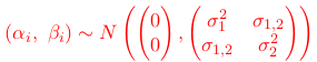
One byproduct of the assumptions above is that observations from the same subjects are correlated. To see this we show that correlation between observations on the same i subjects collected at different time points (t1 and t2) is not 0.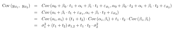
where we used the fact that the errors have mean 0 and are independent of the random effects. For this reason the random effects models are used to model correlated data. The Mixed Effects models are also used for clustered data in general, not only longitudinal data.
The general form of the Linear Mixed Effects Model (LMM) is:
$$ y = X\beta + Z\gamma + \epsilon$$
where y is the dependent variable (outcome), X is the matrix of predictor variables, Z is a design matrix, beta is a vector of fixed effects, gamma is a vector of random effects, and epsilon is a random error which follows a normal distribution with mean 0.
The Generalized Linear Mixed Effects Models (GLMM) extend the LMM by allowing the response variables to follow any distributions from the exponential family (which includes the normal distribution). In addition, a link function is allowed to link the mean of the outcome (mu) to covariates and random effects. The linear predictor in this example includes both the fixed and random effects.
$$ \eta = X\beta + Z\gamma $$
We then assume that \(g(\mu) = \eta \)
Even though the outcome distribution can be chosen to be different from normal, the distribution of random effects is almost always made to be normal.
We below consider a mixed effects Poisson model with a log link fit to the model with a random intercept and fixed effects for time, treatment, baseline and age.
/***** GLMM Model ***********/
title1 ' A GLMM model with a time independent treatment effect';
proc glimmix data=seizures;
  class  id time treatment;
  model RESPONSE=TIME TREATMENT BASELINE AGE/ s d=poisson link=log;
  random intercept /subject = id ;
  estimate 'TRT 1 vs. 0'  TREATMENT -1 1/exp cl;
run;
quit;
The results are similar to the results from GEE. But the two do differ as they are different models. In terms of the interpretation of the coefficients, there is a difference in the case of non-linear models. One difference between GEE and GLM is that GEE estimates population-average while GLMM is the subject-specific effect. These are the same in linear models, but not in non-linear as above.