Bayesian Modeling in Biomedical Research

• Introduction to Bayesian Modeling
• Bayesian Logistic Regression
• Bayesian Linear Regression
• Hierarchical Models

Introduction to Bayesian Modeling

In the frequentist approach, estimated probabilities are viewed as one of an infinite sequence of possible data of the same experiment, while Bayesian analysis is based on expressing uncertainty about unknown quantities as formal probability distributions.

Bayes Problem: Given the number of times in which an unknown event has happened and failed - Requires the chance that the probability of its happening in a single trial lies somewhere between any two degrees of probability that can be named.

Bayesian statistics used probability as the only way to describe uncertainty in both data and parameter. Everything that is not known for certain are modeled with distributions and treated as random variables. Bayesian inference focuses on the uncertainty in value of parameter and decisions which is conditional on sample data.

	Exposed	Unexposed
Diseased	a	b	m1
Not Diseased	c	d	m0
	n1	n0	n

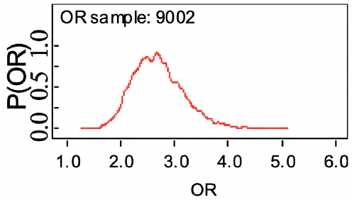
Recall the odds ratio (OR) is the probability of having an outcome (disease) compared to the probability of not having the outcome: ad / bc

Bayesian Statistics takes the point of view that OR and RR are uncertain unobservable quantities, which we can model with a probability distribution.

Prior probability: Model/probability distribution using existing data/knowledge
Posterior probability: Updated model with new and prior data; These are used in inference

Bayes theorem allows us to learn from experience and turn a prior distribution into a posterior distribution.

Bayes Theorem

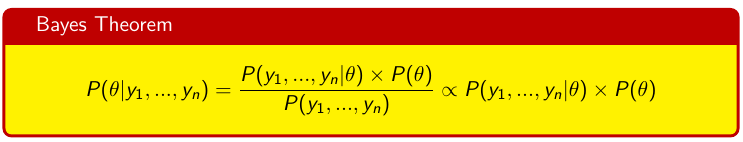
The denominator in Bayes Theorem is a normalizing constant. If a conjugate of the family of distribution then the normalizing constant can be derived.

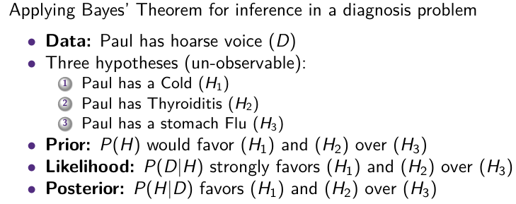
P(H) = Probability of H (Prior Density)
P(H | data) =( P(data | H)*P(H) ) / P(Data) = Posterior probability of H

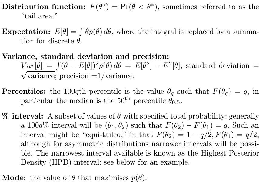
Consider a generic probability distribution p(𝜃) for a single parameter 𝜃. The probability distributions are defined as:

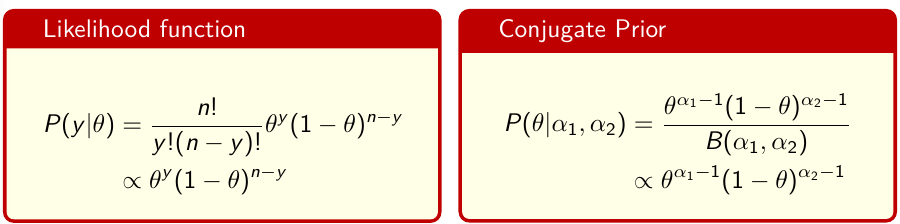
Conjugate Analysis: Beta-Binomial

In conjugate analysis the prior density for theta has the same functional form as the likelihood function.

Credible Interval

A Confidence Interval represents uncertainty we have about the method used in generating an interval that captures the true value in repeated sampling. The parameter is fixed and the interval is random.

A Credible Interval is a statement about the probability that a parameter lies in a fixed interval. The uncertainty is related to the value of the true parameter and the interval is fixed.

Markov Chain Monte Carlo (MCMC) Simulation

There are several ways to calculate the properties of probability distributions for unknown parameters. We will be focusing on using simulation of the known random variables and estimate the property of interest.

Note that there are entire classes on algorithms used for simulation, we will not go into great depth on the underlying theory.

Monte Carlo algorithms are a broad class of computational algorithms that rely on repeated random sampling to obtain numerical results.

Suppose we have a random variable X which has a probability distribution p(x) and we have an algorithm for generating a large number of independent trials x⁽¹⁾, x⁽²⁾, ... x^(T) . Then:

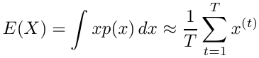
By the law of large numbers the approximation becomes exact as T approaches infinity.

Additionally, if I(l < X < u) is an indicator function where the value is 1 when X lies between l and u and 0 otherwise, the probability can be estimated with Monte Carlo integration by taking the sample average for each realization x^(t)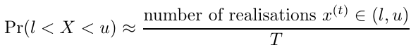

Note that, in general, MCMC methods generate a dependent sample from the joint posterior of interest, since each realisation depends directly on its predecessor. 

In R:

# Step 1: Generate samples
x <- rbinom(1000, 8, 0.5)
# Represent histogram
hist(x, main = "")
# Step 2: Estimate P(X<=2) as
# Proportion of samples <= 2
sum(x <= 2)/1000
## 0.142

Gibbs Sampling

Gibbs Sampling is MCMC algorithm that reduces high dimensional simulation to lower dimensional simulations. Used in BUGS (Bayesian Inference Using Gibbs Sampling) and JAGS as the core algorithm for sampling from posterior distributions.

The algorithm generates a multi-dimensional Markov chain by splitting the vector of random variables θ into subvectors (often scalars) and sampling each subvector in turn, conditional on the most recent values of all other elements of θ. I will not go into great detail on the process because the computer does this for us.

With Gibbs sampling we can give a value to P(𝜃 > .2) or P(Y > 5), but not P(Y > 5 | 𝜃 = .2)

JAGS

JAGS is functionally for the MCMC. It is not a procedural language like R; it can be called from R. You can write complex model code in any order using a very limited syntax

The below code does the same thing as the previous R snippet but using JAGS:

library(rjags)
### model is defined as a string
model11.bug <- "model {
Y ~ dbin(0.5, 8)
P2 <- step(2 - Y)
}"
writeLines(model11.bug, "model11.txt")
# Now run the Gibbs sampling for 1000 iterations
### (Step 1) Compile BUGS model
M11 <- jags.model("model11.txt", n.chains = 1, n.adapt = 1000)
### (Step 2) Generate 1000 samples and discard
mcmc_11 <- update(M11, n.iter = 1000)
### (Step 3) Generate 10000 samples and retain for
### inference
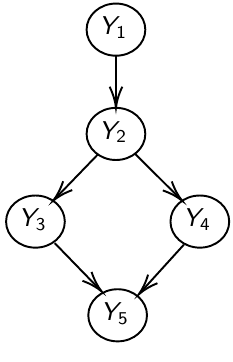
test_11 <- coda.samples(M11, variable.names = c("P2", "Y"), n.iter = 10000)

JAGS uses directed graphical models for internal representation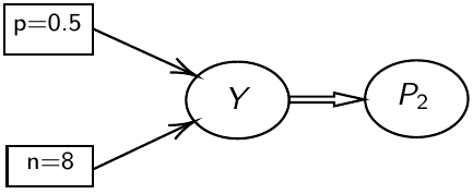

• Nodes represent variables
  
• Directed arrows represent conditional probability distributions
• Double arrows are mathematical functions

The joint probability distribution can be derived using Markov properties of marginal and conditional independence (next section).

Beta Distribution

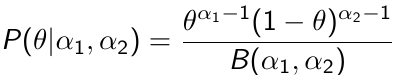
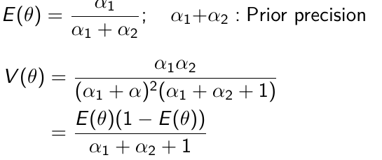
Beta is a family of probability distributions with support between 0 and 1, it is the typical choice for working with probability parameters. The density function depends on two hyper-parameters 𝛼₁ and 𝛼₂.

𝛼₁ + 𝛼₂ = effective sample size with 𝛼₁ events (more on this in a later section)

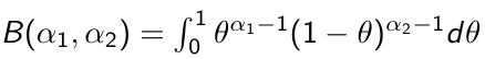
Functions rbeta(), dbeta(), qbeta(), pbeta() available in R for working with Beta distributions. It's also implemented in JAGS as function dbeta( , )

The prior hyper-parameters determine the expected Y events. The posterior mean thus be written as: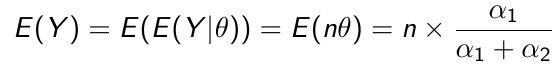

Bayesian Logistic Regression

Let Y be an indicator for presence of disease ->    Y | p ~ Bin(p, 1)

Logistic regression models the log-ODDS (also called logit) of the mean outcome using a linear predictor.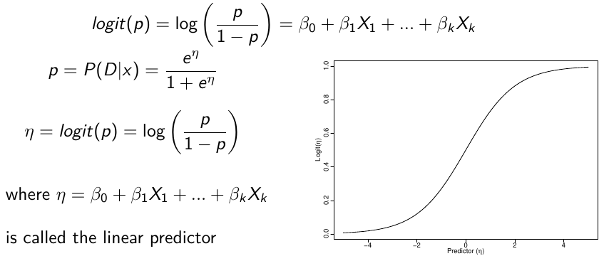

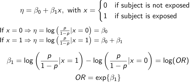
In a case-control study beta_0 is not interpretable. But the estimate of log(OR) can be interpreted correctly, given the symmetry of roles of disease/exposure

H₀: OR = 1; Log(OR) = 0; No association
H₁: OR != 1; Log(OR) != 0; Significant association

The Frequentist approach to test the above is to fit a logistic regression in R using the function glm() and assess the OR.

In Bayesian formulation we need to identify the parameters in our prior model, and the parameters we wish to estimate to form a posterior distribution to assess the OR. We can compute the probability that OR > 1, < 1 or != 1 using a small range.

Ex. Below we model 2 parameters, beta_0 and beta_1, in a DAG model: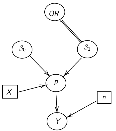

Because there's no constraint on the beta regression parameters, it is common to assume a normal distribution.
The magnitude of variance reflects the amount of uncertainty

In the below code:

• We loop to specify each observation
• Y.D[i] =
  • 1 if subject i has the disease
  • 0 if subject i does not have the disease
• X.E[i] =
  • 1 if subject i has been exposed
  • 0 if subject i has not been exposed

# Analysis with JAGS
library(rjags)

model.1 <- "model{
### data model
for(i in 1:N){
    Y.D[i] ~ dbin(p[i], 1)
    logit(p[i]) <- beta_0 + beta_1*X.E[i]
}
OR <- exp(beta_1)
pos.prob <- step(beta_1)
### prior
beta_1 ~ dnorm(0,0.0001)
beta_0 ~ dnorm(0,0.0001)
 0 i th subject unexposed
}"
# In R Data stored as a list
data.1 <- list(N = 331, X.E = X.E, Y.D = Y.D)
# Compile model (data is part of it!); `adapt` for 2,000 samples
model_odds <- jags.model(textConnection(model.1), data = data.1,
n.adapt = 2000)
update(model_odds, n.iter = 5000) # 5,000 burn-in samples
# Get 10,000 samples from the posterior distribution of OR, beta_0,beta_1
test_odds <- coda.samples(model_odds, c("OR", "beta_1", "beta_0"), n.iter = 10000)
plot(test_odds)
summary(test_odds)

In the output, we'll often look for the point estimate to be the posterior mean. However, when posterior density is skewed, posterior median is sometimes preferable.

Asymptotic Approximation

When the sample size is large enough, one can use an asymptotic approximation of the posterior distribution of the parameters.

When the sampling distribution is a member of the exponential family (Normal, Binomial, Poisson, or Gamma), then the posterior distribution of the parameters is (approximately) normally distribution: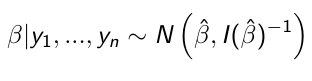
[1]
beta_hat is the ML (maximum likelihood) estimate of beta
I(beta_hat)^-1 is the Fisher Information matrix, evaluated in the ML estimate of beta

Based on the Maximum likelihood theory, asymptotically:
[2]

We don't need a prior in [1] because we have a lot of data. Results in [1] and [2] are close because the prior is weighted low because of the high sample size.

Gibbs Sampling for Logistic Regression

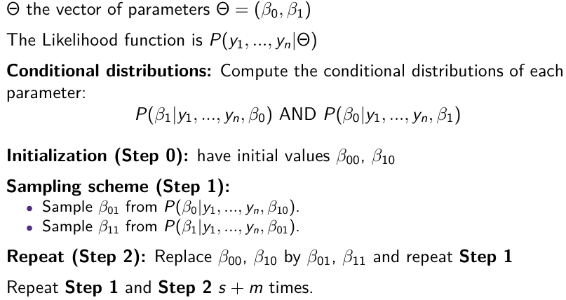
Posterior Inference

Obtain s + m sample for each parameter
Throw away the first s values (burn-in)
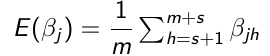
Use the m samples with Monte Carlo algorithms to carry out inference:

1. Point Estimates - Posterior means or medians
   

   

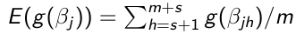
2. Transformations - Any function of the parameters
   

   

3. Posterior Density - Density estimation methods to estimate the posterior density of parameters
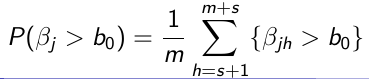
4. Tail probabilities
   

   

Marginal and Conditional Independence

Two random variables, X and Y, are independent (denoted by X ⊥ Y) if an only if:
P(X, Y) = P(X)P(Y); Joint p.m.f. for joint density = Marginal p.m.f. or marginal density

Given three random variables, X, Y and X, are conditionally independent given Z (denoted by Y  ⊥  Y | Z) if and only if:
P(X, Y | Z) = P(X | Z) P(Y | Z)

There is no relation between marginal and conditional independence (Simpson Paradox)

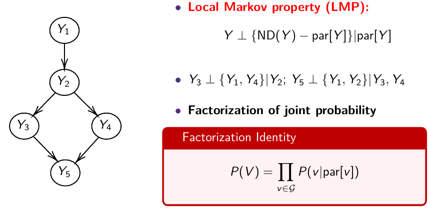
The directed graph specifies conditional and marginal independence through two properties; The Local Markov Property (LMP) specifies that we need to specify only the distribution of nodes given their parents. The Global Markov Property (GMP) is used internally to derive the conditional distributions of each node given all others.

Local Markov Property (LMP)

Descendants of Y [D(Y)] are all nodes reached from Y with a directed path
Non-descendants of Y [NS(Y)] - all nodes minus the descendant nodes

Global Markov Property (GMP)

The node is independent of everything else in the network given its Markov Blanket.

For each node, list the Markov blanket: Markov blanket of A: the parents of A, the children of A and the parents of the children of A

Y_1 independent of Y_3, Y_4, Y_5, given Y_2
MB(Y_1) = { Y_2 }; MB(Y_2) = { Y_1, Y_3, Y_4 }

The LMP is used to specify the priors and the likelihood
The GMP is used to generate the conditional distributions to run the Gibbs Sampling

Bayesian Hypothesis Testing: Prior Odds

On each hypothesis we  have a prior probability:
P(H₀) = P(M₀) and P(H_a) = P(M₁)

Use the data to compute the posterior probability of each hypothesis: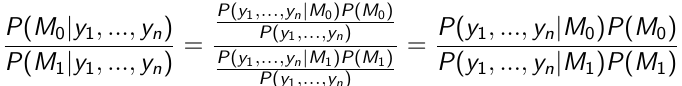

This equates to:
Posterior ODDs = Bayes Factor * Prior Odds
We accept the hypothesis with maximum posterior probability (0 - 1 loss)

The Bayes Factor is the ratio of the likelihood functions computed for models M0 and M1

If P(M0) = P(M1) then the posterior probability of M1 is larger than the posterior probability of M0

We can also assign weights to adjust the probability of making errors: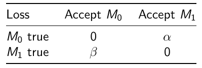

Where alpha would be the loss incurred if M1 is accepted when M0 is true
and beta is  the loss incurred if M0 is accepted when M1 is true.

Bayesian Linear Regression

By now we know what a linear regression looks like. Let's consider a special case where number of parameters, p = 0: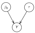

Assume Y is distributed as a normal distribution with mean β₀:
Y|β₀, τ ∼ N(β₀, σ² = 1/τ )

τ = 1 / σ² , also called precision   <- Be aware this will be used interchangeably with variance

The density function is: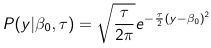

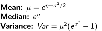
Mean and variance:
E(Y) = μ₀; V(Y) = 1/τ₀ + τ

The Posterior Distribution for β₀ is calculated using Bayes' Theorem

When Mean and Variance are Unknown

We use a Normal prior distribution for the mean β₀ ∼ N(μ₀, τ₀) and a Gamma prior distribution for the precision parameter: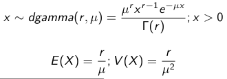

JAGS example:

model.1 <- "model {
	for (i in 1:N) {
		hbf[i] ~ dnorm(b.0,tau.t)
	}
	## prior on precision parameters
	tau.t ~ dgamma(1,1);
	### prior on mean given precision
	mu.0 <- 5
	tau.0 <- 0.44
	b.0 ~ dnorm(mu.0, tau.0);
    
    ### prediction
	hbf.new ~ dnorm(b.0,tau.t)
	pred <- step(hbf.new-20) # hbf >= 20
}"

Predictive Distributions

Given the Prior and Observed data we can compute the probability of a new observation will be greater or less than some integer threshold. The predictive distribution is a distribution of unobserved y^~, that is: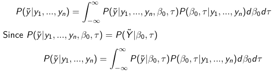

The two sources of variability in prediction are in the parameters V(β₀, τ | y) and the variability in the new observation V(y | β₀, τ)

• To simulate from predictive density, do repeatedly:
  1. Sample one sample β₀^*, τ* from posterior β₀, τ | y
  2. Sample one y^~ ~ N(β₀^*, 1/τ* )
•  During the Gibbs sampling we generate samples values from the posterior distribution β₀, τ | y
•  So Generating y^~ ~ N(β₀, τ | y) will produce the correct predictive distribution samples. P(y^~ > 20 | data) is the proportion of y^~ > 20

Log Normal Distributions

Since in the example above the outcome distribution can only be positive we can use a Log-Normal distribution, a continuous distribution with support for values y > 0.

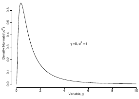
Y | η, σ² ~ INormal(η, σ²) with density function: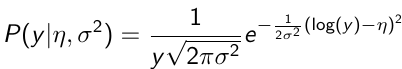

It also implies:     Log( Y )~ Normal(η, σ²)

In JAGS we use: dlnorm(η, σ²)

"model {
for (i in 1:N) {
	hbf[i] ~ dlnorm(lb.0,tau.t)
}

## prior on precision parameters
tau.t ~ dgamma(1,1);

### prior on mean
lb.0 ~ dnorm(1.6,1.6);

b.0 <- exp(lb.0)

### prediction
hbf.new ~ dlnorm(lb.0,tau.t)
pred <- step(hbf.new-20)
}"

In the above example, we get the initial prior on β₀ from previous data, where we derived median(b.0)=5 and V(b.0)=1/0.44=2.27
Then we take the log of the median to get η and transform the precision variable with:  log(1 + V (b.0)/E (b.0)² ), then take the inverse of that to get the variance.

Parameter Interpretation

Let's consider data of the SNP rs766432 on the effect of HbF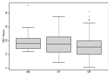

Where HT is heterzygote, HM is homozygoute and NP is common alleles.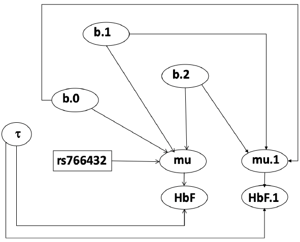

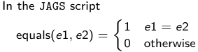
• We start by creating indicators for HT and NP using the equals( , ) function in JAGS
  
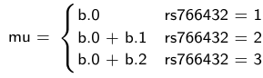
• The mean of Log HbF
  
  b.1 = the effect of HT vs HM
  b.2 = the effect of NP vs HM
• The hypotheses:
  1. H0: b.1 = 0; HM and HT have the same effect
  2. H0: b.2 = 0; HM and NP have the same effect

model.1 <- "model {
	for (i in 1:N) {
		hbf[i] ~ dlnorm(mu[i],tau.t)
		mu[i] <- b.0+b.1 *equals(rs766432[i],2)+b.2 *equals(rs766432[i],3)
	}
	## prior on precision parameters
	tau.t ~ dgamma(1,1);
	### prior on mean given precision
	b.0 ~ dnorm(0, 0.001);
	b.1 ~ dnorm(0, 0.001);
	b.2 ~ dnorm(0, 0.001);
	### prediction
	lmu.1 <- b.0;
 	hbf.1 ~ dlnorm( lmu.1,tau.t); 
    pred.1 <- step(hbf.1-20)
	lmu.2 <- b.0+b.1; 
    hbf.2 ~ dlnorm( lmu.2,tau.t); 
    pred.2 <- step(hbf.2-20)
	lmu.3 <- b.0+b.2; 
    hbf.3 ~ dlnorm( lmu.3,tau.t); 
    pred.3 <- step(hbf.3-20)
	### fitted medians by genotypes
	mu.1 <- exp(lmu.1)
	mu.2 <- exp(lmu.2)
	mu.3 <- exp(lmu.3)
	par.b[1] <- b.0;
	qpar.b[2] <- b.1;
	par.b[3] <- b.2
	par.h[1] <- hbf.1; 
    par.h[2] <- hbf.2; 
    par.h[3] <- hbf.3;
	par.m[1] <- mu.1;
	par.m[2] <- mu.2;
	par.m[3] <- mu.3
	par.p[1] <- pred.1; 
    par.p[2] <- pred.2; 
    par.p[3] <- pred.3
}"

data.1 <- source("saudi.data.2.txt")[[1]]
model_hbf <- jags.model(textConnection(model.1), data = data.1,n.adapt = 1000)
update(model_hbf, 10000)
test_hbf <- coda.samples(model_hbf, c("par.b", "par.h", "par.m","par.p"), n.iter = 10000)
summary(test_hbf)
plot(test_hbf)
autocorr.plot(test_hbf)

To analyze the convergence we can observe normality in auto-correlation plots. If we wee substantial auto-correlation (lag > X), we can repeat the the MCMC for 100,000 simulations and sample every X steps by using thin = X in coda.samples(); where X is how often order occurs in the plot.

test_hbf <- coda.samples(model_hbf, c("par.b", "par.h", "par.m","par.p"), n.iter = 1e+05, thin = 30)

Depending on which hypothesis we are testing we could also eliminate b.1 or b.2. Or in other situations reparameterizations can reduce correlation.

ANOVA Example

In this example let's consider a study of 5 different treatment groups assigned to wear shirts with differing levels of cotton (15%, 20%, 25%, 30%, and 35%) and strength was measured. We'll code these levels as dummy variables and

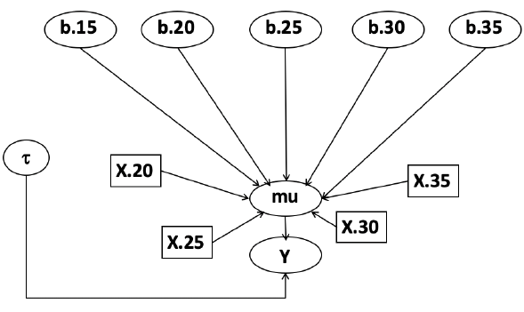
Note that since 15% is the reference group we keep it as a constant.

model.1 <- "model {
	### data model
	for(i in 1:N){
		y[i] ~dnorm(mu[i], tau)
		mu[i] <- b.15 + b.20*lev.20[i] +b.25 *lev.25[i] +
		b.30*lev.30[i] +b.35 * lev.35[i] 
    }
	###
	prior
	b.15 ~dnorm(0,0.0001); ## referent group
	b.20 ~dnorm(0,0.0001);
	b.25 ~dnorm(0,0.0001);
	b.30 ~dnorm(0,0.0001);
	b.35 ~dnorm(0,0.0001);
	tau ~dgamma(1,1)
	### difference in strength between level 3 (25%) and level 4 (30%)
	b.30.25 <- b.30-b.25
	### estimated strength in groups (30%)
	strength[1] <- b.15
	strength[2] <- strength[1]+b.20
	strength[3] <- strength[1]+b.25
	strength[4] <- strength[1]+b.30
	strength[5] <- strength[1]+b.35
}"

ANCOVA Example

These are models that include a continuous covariate and a categorical variable with 2 categories.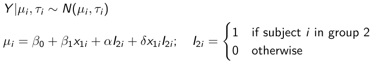

When the slope differs in the 2 groups and the lines are not parallel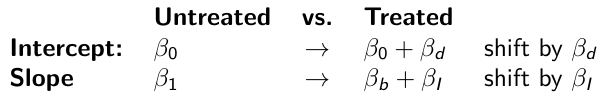

model.1 <- "model{
  ### data model
  for(i in 1:N){
      hbf_after[i] ~dlnorm(mu[i],tau)
      Lhbf_baseline[i] <- log(hbf_baseline[i])
      mu[i] <- beta.0 + beta.d*Drug[i] +
      beta.b*(Lhbf_baseline[i]-mean(Lhbf_baseline[])) +
      beta.i*Drug[i] *(Lhbf_baseline[i]-mean(Lhbf_baseline[]))
  }
  ### prior density
  beta.0 ~ dnorm(0,0.0001)
  beta.d ~dnorm(0, 0.0001)
  beta.b ~dnorm(0, 0.0001)
  beta.i ~dnorm(0,0.0001)
  tau ~ dgamma(1,1);
  ### inference
  parameter[1] <- beta.0
  parameter[2] <- beta.d
  parameter[3] <- beta.b
  parameter[4] <- beta.i
}"
### generate data
Drug = rep(0, nrow(hbf.data))
Drug[treatment == "Hy"] <- 1
table(Drug, hbf.data$Drug)
data.1 <- list(N = as.numeric(nrow(hbf.data)), hbf_baseline = hbf_baseline, hbf_after = hbf_after, Drug = Drug)
model_mean <- jags.model(textConnection(model.1), data = data.1,n.adapt = 1000)
update(model_mean, 10000)
test_mean <- coda.samples(model_mean, c("parameter"), n.iter = 10000)

So if the interaction term is significant then we would conclude the treatment has an effect

Missing Values

Treat missing values in the response as unknown parameters and JAGS will generate them as a form of imputation. Missing data in the covariates however is not so easy.

Model Selection: DIC

• Model selection based on marginal likelihood is most robust but difficult to implement
• Often model search over many models is based on BIC using posterior estimates of parameters
• Model selection for a small number of models is based on posterior intervals

Start from the deviance: -2log(P(y | β, τ ))

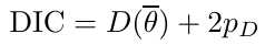
Deviance information Criterion:
DIC = Dbar + pD = Dhat + 2 * pD

Dbar: -2 E(log(P(y | β, τ ))) = posterior mean of the deviance
Dhat: -2 log(P(y | β^, τ^ ) = point estimate of the deviance using the posterior means of the parameters
pD: Dbar - Dhat = Effective number of parameters

The model with the smallest DIC is estimated to be the model that would best predict a replicate dataset of the same structure as the observed.

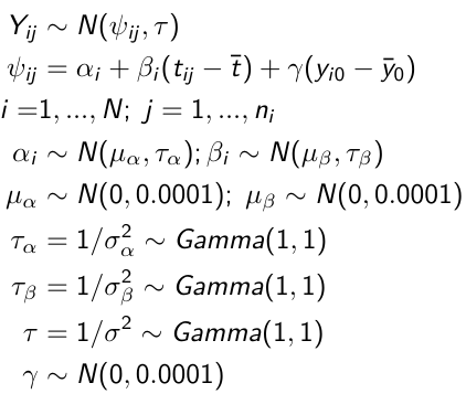
Hierarchical Models

Previously we have assumed given covariates, the observations are independent. However, there are many situations where this does not hold. Bayesian Hierarchical models can be used to cluster observations, where each cluster might have its own cluster-specific parameters.

In Bayesian hierarchical models, we start by imposing a prior that is a function of different parameters. We'll introduce a new variable γ, which is called the hyper-prior; The prior of α depends on β, which depends on γ.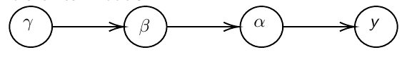

Hyper-parameters: Parameters of prior distribution
Hyper-Priors: Distribution of Hyper-parameters

A typical example of this in medical research is population of hospitals, providers within hospitals, and patients within providers. Any datasets with such a structure are called hierarchical. Hierarchical models are also called partial pooled or random effect models.

We are interested in making inference of specific units. In doing so observations may be collected over time on the same individuals, so repeated measures must be accounted for.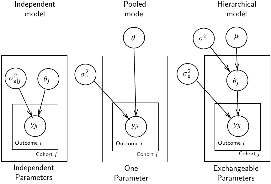

• Independent models have no randomly-varying effects
• Pooled models have a randomly-varying (subject-specific) effects of slope
• Hierarchical h ave randomly-varying (subject specific) effects of slope and intercept

Ranking Posterior Estimates

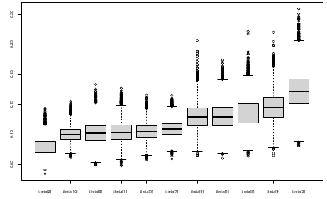
We can simply rank the outcome/results in a box plot such as the above, but this does not consider the uncertainty of the estimates.

We can derive the posterior distribution of each ranking by ranking the estimates at each iteration of the Gibbs Sampling and generate the posterior distributions of the ranks. Below the ranks are in parenthesis: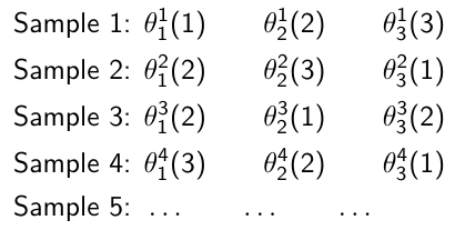

The posterior distribution of ranks gives us a measure of the uncertainty of the ordering.

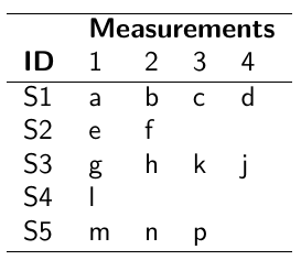
Data Formatting

There are three main alternative approaches to account for the hierarchical structure of the data in coding, in order of popularity:

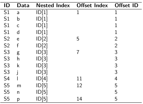
1. Nested Indexes - Define an index of the same length of the data that specifies the cluster to which each unit belongs.
2. Offset - Construct a vector of indexes that define the first and last element of each cluster. Needs two indexes
   

   Tabular Format: Long Format:

3. Data padding - Structure data in array format and fill in empty cells with NA when clusters include different sample sizes

Model Implementation With Offset

### Begin by setting up the data and generating the offset
## Prepare outcome and covariate data
y <- na.omit(c(t(HB.data[, 6:8]))) # All outcome data
y0 <- HB.data[, 5] # Baseline data
t <- c(t(HB.data[, c(2, 3, 4)]))[-na.action(y)] # Times corresponding to non-missing outcome

## Fill in data for offset indexes one subject at a time, starting with the first subject
i <- 1
offset <- c(1, 1 + length(which(is.na(HB.data[1, 6:8]) == F)))

## Add a new offset for each subject until the end of data
while (offset[(i + 1)] < length(y) - 1) {
	i <- i + 1
	offset <- c(offset, offset[i] + length(which(is.na(HB.data[i,6:8]) == F))) # Calculate offsett for subject i
}
offset <- c(offset, (length(y) + 1)) # Concatenate to the set of offsets

model.1 <- "model {
	for (i in 1:N) {
		for(j in offset[i] : (offset[i+1]-1)){
			y[j] ~ dnorm(psi[j], tau.y)
			psi[j] <- alpha[i] + beta[i]*(t[j] - tbar)
				+ gamma*(y0[i] - y0bar)
		}
	alpha[i] ~ dnorm(mu.alpha, tau.alpha)
	beta[i] ~ dnorm(mu.beta, tau.beta)
	}
	# priors
	sigma.a <- 1/tau.alpha
	sigma.b <- 1/tau.beta
	sigma.y <- 1/tau.y
	mu.alpha ~ dnorm(0, 0.0001)
	mu.beta ~ dnorm(0, 0.0001)
	gamma ~ dnorm(0, 0.0001)
	tau.alpha ~dgamma(1,1)
	tau.beta ~dgamma(1,1)
	tau.y ~dgamma(1,1)
	y0bar <- mean(y0[])
	tbar <- mean(t[])
}"

i = subject
offset[i]: (offset[i + 1] -1) = observations corresponding to subject i

Checking Convergence

The major assumption of MCMC is convergence. There are 4 widely-used diagnostic plots in R:

• Gelman and Rubin: With M >= 2 chains calculate the potential scale reduction factor as ratio of estimated variance of the parameter and within-chain variance
• Gewke: Test for equality of means between two non-overlapping parts of the Markov Chain
• Raftery and Lewis: Calculates the number of iterations N and the number of burn-ins M necessary for a quantile of interest q to be estimated with an acceptable tolerance r (in (q-r, q+r)) with a probability s
• Heidelberg and Welch: Calculates a test statistic to test the null hypothesis that the Markov chain is from a stationary distribution

Gelman and Rubin Diagnostics

With m chains of length n, GR convergence diagnostic provides numeric convergence summary based on multiple chains (at least 3 chains are required)

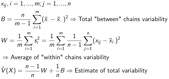
If the chains are all from stationary distributions: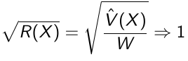

jags.snp <- jags.model(textConnection(model.snp), data = data.snp, n.adapt = 1500, n.chains = 3) 
update(jags.snp, 1000)
test.snp <- coda.samples(jags.snp, c("beta.snp"), n.iter = 1000)
geweke.diag(test.snp, frac1 = 0.1, frac2 = 0.5)
gelman.diag(test.snp)
gelman.plot(test.snp, ylim = c(1, 4))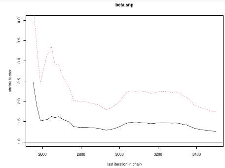

This graph is an example of chains that do not converge; They could be approaching 1 but we see a lot of variability especially near the beginning.

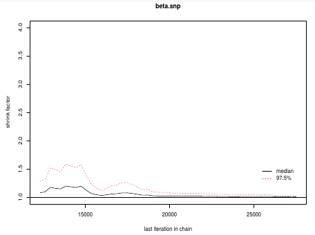
In this plot we can observe the lines converge around 1.

Note: Parallel Computing

As the number of chains for convergence increases in more complicated models we require more computing power. There are several packages in R that can be used to do this, perhaps the most used being snowfall or doParallel.

Comparing Hierarchical Models

Joint likelihood of data and parameters:

There are three primary approaches used:

• Deviance Information Criterion (DIC)
  

  
  Which is based on p(y | θ)
  

• Akaike Information Criterion (AIC)
      AIC = -2 log(y | φ̂) + 2p_φ
  where p_φ is the number of hyper-parameters
  
• Bayesian Information Criterion (BIC)
      BIC = -2 log(y | φ̂) + log(n)*p_φ

"Likelihood" is not well defined in a hierarchical model; It depends on the "focus" of the study if we want to use θ, φ, or the model structure without any unknown parameters. It is not a matter of which is correct but which is appropriate for our purpose.

Consider an example where our model predicts classes within schools in within a country:

• If we are interested in predicting future classes in those school then θ is the focus and deviance-based methods such as DIC are appropriate
• If we are interested in predicting results of future schools in a country then φ is the focus and marginal-likelihood methods such as AIC are appropriate; Relevant to education within the whole country.
• If we are interested in predicting results for a new country, then no parameters are in focus, the Bayes factors are appropriate to compare models; Relevant to general statements about education in the
• whole world or outside of the country being studied.

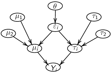
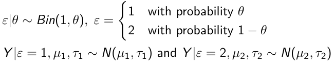
Mixture Models

Mixture models integrate multiple data generating processes into a single mode; AKA a mixture of many distributions. This is especially useful in cases where the data doesn't allow us to fully identify which observations belong to which process, such as clustering.

model.1 <- "model{
p[1] <- theta
p[2] <- 1 - theta
for( i in 1 : N ) {
	epsilon[i] ~ dcat(p[]) # dcat: categorical outcome
	y[i] ~ dnorm(mu[epsilon[i]],tau[epsilon[i]])
}
theta ~ dbeta(1,1)
for (j in 1:2){
	mu[j] ~ dnorm(0.0, .0000001);
	tau[j] ~ dgamma(1,1)
	sigma[j] <- pow(tau[j],-2)
}
}"

 ε value hidden → two profiles