Applied Statistics in Clinical Trials
BS851: Statistical research design considerations, including randomization and sample size
determination, and methods for analyzing and interpreting statistical results from clinical trials.
- Introduction to Clinical Trials
- Randomization of Subjects
- Continuous and Binary Endpoints
- Baseline Variable Adjustment
- Survival Analysis in Clinical Trials
- Multiple Comparisons
- Non-Inferiority in Clinical Trials
- Effect Modification and Interaction
- Interim Analysis and Data Monitoring
- Correlated Data in Clincal Trials
Introduction to Clinical Trials
A clinical trial is defined as a prospective study comparing the effect or value of an intervention against a control in subjects. The core components of clinical trials are the population, intervention, control and outcome. The great majority of clinical trials are concerned with the evaluation of drug therapy, but intervention could be anything.
The steps in creating a clinical trial:
- Research question
- Design the trial (protocol)
- Enrollment/Data collection and check
- Conduct the trial
- Data freeze
- Data analysis
- Interpret results
Clinical Equipoise
The genuine uncertainty within the scientific and medical community as to which of the two interventions is superior.
FINER Criteria
- Feasible (is it possible?)
- Interesting
- Novel (is it new?)
- Ethical - always the most important
- Relevant (does it matter now?)
Belmont Principles
Relevant to the ethics of research involving human subjects:
- Respect of persons - informed consent
- Beneficence - to do no harm
- Justice - Fairness among those chosen for the study
Possible Objectives of the Intervention
The new experimental intervention being tested usually has one of the following primary objectives:
- Cure a disease
- Reduce disease symptoms
- Prevent disease worsening
- Prolong survival time (terminal disease) or prevent disease (vaccine)
- etc.
Types of Intervention Studies
- Pharmaceutical products
- Synthetic drugs
- Biologics
- Products made from human or animal cell/tissue such as vaccines or blood replacement products
- Medical Devices
- Pacemaker, cardiac stents, etc
- Other (education, exercise, therapy, etc)
Case-Control Experiments
Blinding ensures patients and/or investigators and/or analysts don't know which treatment is assigned to whom. It is not always possible to blind a study.
- Single-blind: One group does not know treatment assignment
- Double-blind: Two groups do not know treatment assignment (usually the subject and investigator)
- Open-label: Patient and investigators know the treatment
Placebo Control
A placebo is made of something that shouldn't have an effect on the body and is useful in determining if an intervention is "better than nothing". A placebo control theoretically has no physical effect on the disease, but it may have a psychological effect.
Active Control
Sometimes it is best to compare a new product to the currently marketed treatment or "standard of care". This would be preferable in control groups for terminal diseases, where it would be unethical to give a placebo.
Randomization
Allocation of the subject to one the interventions by chance. Yields the highest probability that treatments have a balanced distribution on measured and unmeasured covariates related to the outcome.
Non-Compliance in Clinical Trials
Some individuals never receive treatment to which they were randomized, stop treatment, or fail to consistently take treatment. We must consider how we approach this in our analysis:
- Intention to treat: Compare randomized groups regardless of compliance (usual primary approach)
- Modified intention to treat: Exclude patients who were randomized but not eligible or did not have any post-baseline data
- Per-protocol: Compare only individuals who took the medication and/or are compliant with the assigned treatment and were eligible
Study Designs
Parallel Group Design
Most common design and the main focus of this course. Multiple treatment groups and subjects are randomized to exactly 1 treatment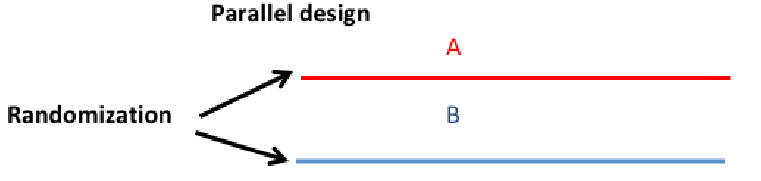
Crossover Design
Each patient is randomized to a random sequence of treatment that will be administered sequentially. The objective remains to compare treatment A vs B. Typically less individuals are required.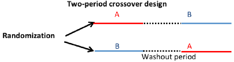
Factorial Design
Often researchers are interested in studying the effect of two or more interventions applied alone or in combination.
Ex. 2x2 factorial design in which two interventions in A and B are evaluated
| (left is A, top is B) |
- |
+ |
| - |
Control |
B only |
| + |
A only |
A and B |
Study Protocol
Every trial has a written protocol, documenting all information concerning the purpose, the design, conduct of the trial and data analysis. This promotes good faith by stating what data is collected and for what purpose, and facilitates communication with relevant ethics committee or regulatory bodies and the sponsor.
Investigators are expected to summarize the study design, regularly provide updates on recruitment and submit results.
- Administrative information
- Title, trial registration, protocol version, funding, roles and responsibilities
- Introduction
- Background
- Research hypotheses
- Study design
- Methods
- Settings and recruitment
- Eligibility criteria
- Treatment/interventions
- Primary outcome
- Timeline
- Sample size considerations
- Treatment allocation, randomization and blinding
- Data collection and data management
- Statistical analysis plan
- Data monitoring and auditing
- Ethics, ethics approval, protocol amendments, consent, confidentiality, declaration of interests, access to data, post-trial care and dissemination policy
Every clinical trial regardless of the sponsor must be registered at clinicaltrials.gov
Key Players in Regulatory Approval
- Patients
- Informed consent required for all study participants
- Sponsor
- Pharmaceutical industry, government agencies, research institutions, health maintenance organizations, or insurance companies
- Investigators
- Study team, including statisticians and clinical coordinators
- Regulatory agency
- FDA in US, EMEA in EU
Clinical Research for Drug and Device Trials
The average time a pharmaceutical company
spends to get a drug on the market is 15 years; 6.5 years in pre-clinicals and discovery, 7 years in clinical trials, 1.5 years review time at FDA.
Pharmacokinetics how the drug flows through body and how it is excreted
Pharmacodynamics how drug affects the body
- Sponsor and submit IND application to FDA
- Phase 1: First time in humans
- Goal: Assess the safety and determine the metabolism of the drug in humans - usually no interest in efficacy
- Sample size: 20-80 healthy volunteers, unless the treatment is for a life-threatening disease
- Typically exposed to increasing doses to determine maximum tolerated dose (MTD)
- There are concerns about exploitation for participants who underestimate the risk vs reward
- Phase 2: Exploratory
- Goal: to investigate short term safety and efficacy of the drug in patients with the disease that the drug is intended to treat
- Sample size: 50 - 300 patients
- Focus on dose-response relationship, usually case-control with a placebo for non-serious diseases and active-control for serious diseases
- Phase 3: Pivotal, Confirmatory
- Goal: Confirm the efficacy of the new drug while assessing safety. Final stage before drug is licensed
- Sample size: based heavily on statistics, sample must be large enough to detect clinically relevant effect
- Patients are randomized to usually one dose of experimental product vs one control
- Phase 4: Post-license monitoring
- Focus: Establish long-term efficacy and safety of the drug after the drug has been licensed
- Sample size: Similar to phase 3
- Evaluated long period of time in a large number of patients, the difference from phase 3 is these trials tend not to be placebo controlled.
FDA usually requires at least 2 adequate well controlled trials conducted in humans to demonstrate substantial evidence of effectiveness and safety. Exceptions are made for serious or immediately life-threatening disease with no therapy available, approval can be granted based on several Phase 2 trials or surrogate outcomes.
The "International Conference on Harmonisation" (ICH) is a conference of professionals from Europe, Japan, and US to determine guidelines related to the conduce and design of pharmaceutical/biotech clinical trials.
Randomization of Subjects
Subjects are assigned to study groups by a random mechanism not controlled by the patient or the investigator. Randomization increases the likelihood treatment groups are comparable with respect to distribution of measurable and measurable characteristics.
Randomization Schedule
Prior to study start, a randomization schedule is generated by a statistician. Ex. a 2 treatment trial with 1:1 randomization.
Treatment allocation schemes should:
- Be unpredictable
- Neither the participant nor the investigator know in advance which treatment will be assigned (reduced observation bias)
- Promote balance
- Groups must be alike in all important aspects and only differ in the intervention each group receives
- Be simple
- Easy for investigator/staff to implement
Generally, the randomization ratio should be equally allocated (1:1 randomization). Unequal randomization arises in some situations where we want more in one group than another due to costs or other factors.
Methods of Randomization
- Unrestricted randomization
- Block randomization
- Randomized permuted blocks
- Stratification
- Adaptive randomization
- Biased coin, etc
- Minimization
- Cluster randomization
Unrestricted Randomization
- Equivalent to tossing a fair coin for each subject that enters the trial
- Assign each treatment randomly and independently of previous treatment
- Also called simple/complete randomization
SAS Code for generating unrestricted random data:
*Method 1;
*RANUNI: generates random numbers between 0 and 1 which have a uniform distribution;
data one;
seed=123;
do id=1 to 8;
r=ranuni(seed);
if r<0.5 then group='A';
if r>=0.5 then group='B';
output;
end;
run;

* Method 2;
data one;
seed=123;
do id=1 to 8;
r=ranuni(seed);
output;
end;
run;
proc sort data=one;
by r;
run;
data two;
set one;
if _n_<=4 then group='A';
if _n_>4 then group='B';
run;
proc sort data=two;
by id; * Sort again by id;
run;

* Method 3;
data three;
seed=123;
do id=1 to 8;
r=ranuni(seed);
output;
end;
run;
proc rank data=three groups=3 out=three;
var r;
ranks group;
run;
data three;
set three;
if group=0 then trt='A';
if group=1 then trt='B';
if group=2 then trt='C';
run
Note that the seed is a number that determines the starting value. The same positive seed will always generate the same result. If we want a different number each run then set the seed <= 0.
The issue with unrestricted randomization is that is can produce imbalance. Ex. Based on the binomial distribution, a study with two groups and 8 patients will produce a 6:2 assignment 28% of the time.
Block Randomization
Also called permuted block, and is the most common form of randomization in clinical trials. Sequence of blocks that contain the assignment in the desired ratio.
Ex. With N = 8 patients and 2 treatments, A and B, with 1:1 randomization and block size 4:
- Take the letters AABB, randomly permute them
- Assign treatment for the next set of 4 patients, randomly permute AABB again
Block randomization ensures that of the first 4 patients, 2 receive each treatment.
Choosing Block Size
The block size must be a multiple of the number in the allocation ratio. Block size is not always mentioned in the study's protocol, as no one needs to know except the statistician who generates the schedule.
A block size of 2 is usually not recommended. It creates a "guessable" pattern of AB, BA, AB...
A large block size is also not recommended (especially for small samples). May lead to incomplete blocks at the end of the study. Ex. N = 12 with block size 8 would leave 4 incomplete blocks.
Block randomization SAS with 12 patients, 2 treatments and block size 4:
proc plan seed=1133637;
factors blocks=3 ordered trt=4 random/noprint;
output out=randschd trt cvals=('A' 'A' 'B' 'B');
run; quit;

ods rtf file='rand.rtf';
options nodate nonumber;
* Add patient ID ;
data randschd;
set randschd;
patient+1;
run;
* Final randomization schedule;
proc print data=randschd (obs=12)
label noobs;
var patient trt;
label patient='Patient ID’
trt='Treatment';
title1 'Pharmaceutical
Company, Inc. ';
title2 'Protocol XXXXXX
Randomization Schedule';
run;
ods rtf close;
Random Block-Size Randomization
In 'open label' studies there is no concern the investigator might deduce the block size over time.
In this method we choose 2 block sizes and randomly assign a size to each block. Then within each block, randomize patients to treatment using permuted block method. This makes it very difficult to guess the next assignment.
Ex. ABBABA - BABA - AABBAA - BABABA
* Random block with 2 treatments, 20 participants and block sizes of 2 and 4 with 1:1 randomization;
* Step 1: generate blocks of random size;
data blocks;
do block=1 to 10;
	half_size=rantbl(2019,0.5,0.5);
	size=half_size*2;
	do j=1 to half_size;
		do treatment='A','B';
		random=ranuni(2019);
		output;
		end;
	end;
end;
run;

* Step 2: permute the blocks;
proc sort data=blocks;
by block random;
run;
Stratified Randomization
Randomization is performed within strata by one or more subject characteristics. Use a permuted blocks design within each stratum. The goal is to ensure balance within each stratum.
In multi-center studies typically one stratifies the randomization by center.
Too many small strata can defeat the balancing effects of blocking, because you could get imbalances or long runs when you look at the sample as a whole.
- Use a limited number of strata in your randomization
- Consider using regression adjustments later if there are imbalances in baseline factors
The SAS code for 24 participants, 2 treatments, 1:1 randomization and block size 4.
proc plan seed=8894670;
factors site=2 ordered
blocks=3 ordered
trt=4 random/noprint;
output out=randschd2
trt cvals=('A' 'A' 'B' 'B');
run; quit;

* Create unique study ID ;
data randschd2;
set randschd2;
by site;
if first.site then patient=0;
patient+1;
if site=1 then
patid=patient+100;
if site=2 then
patid=patient+200;
run;

*Same as above, but with 2 weight stratum within each of the two sites;
proc plan seed=8894670;
factors site=2 ordered wgt=2 ordered blocks=3 ordered trt=4
random/noprint;
output out=randschd3 trt cvals=('A' 'A' 'B' 'B');
run; quit;

*2:1 Randomization with 18 participants, 2 treatmetns, block size 6 and 2 sites;
proc plan seed=8894670;
factors site=2 ordered wgt=2 ordered blocks=3 ordered
trt=6 random/noprint;
output out=randschd4 trt cvals=('A' 'A' 'A' 'A' 'B' 'B');
run; quit;
Adaptive Randomization
Array of methods to determine treatment assignment aimed at making trials more efficient. Allows to adapt the study design using data accumulated from early stages of the trial.
Two types:
- Based on the previous treatment assignments (e.g. Efron biased coin, minimization)
- Based on previous outcomes
Minimization is an alternative to stratification when the number of strata is large. The procedure is as follows:
- k subjects are randomly assigned to treatment groups A or B
- For each subsequent subject, compute an imbalance score under the two hypothetical treatment assignments A and B
- Assign subject to the treatment allocation with lower score (deterministic approach) or give higher assignment probability to treatment with lower score (probabilistic approach).
The general idea is that as the data accumulates we will tend to assign subjects to the treatment that proves more effective.
'Play the Winner' Randomization Scheme:
- If treatment A is successful based on accumulated data, a new available subject will be given a higher probability of being assigned to A
- If treatment A is not successful then assign to B with higher probability
- Proceed over time until we have enough evidence to make a decision
Pros and Cons:
+ Typically requires fewer subjects (efficiency)
- Special statistical methods
- Unlike permuted blocks, randomization lists cannot be made available before the study and require recalculation of treatment assignment probability with each new subject
Cluster Randomization
In studies of health service implementation or treatment delivery it is often preferable to randomize centers, physicians or communities rather than individual subjects.
Also used when there is the potential for contamination; aspects of intervention adopted by participants in the control group.
Blinding/Masking
Biases may be intentionally or unintentionally introduced into the conduct and analysis of a trial. Personnel and participants may have inherent biases regarding the treatment.
Types of Bias:
- Selection bias: Occurs when the investigator consciously or otherwise uses knowledge of the upcoming treatment assignment to help decide who to enroll
- Observer bias: Occurs when the knowledge of treatment allocation affects the evaluation of the response to treatment
- Ex. A physician knows a patient receives treatment and subconsciously may probe more when evaluating
- Perception bias
- Ex. A patient receives a control subconsciously may be less enthusiastic and under-report
- an efficacious effect.
Blinding is the process of 'hiding' the treatment that a patient receives. When it is feasible, blinding eliminates potential biases.
Types of Blinding:
- Double-blind trial (most common) - Neither the study physician treating/evaluating nor the subject know the treatment patient is receiving
- Single-blind - Treating physician knows, but patient does not know
- Open-label - both subject and investigator know
- Triple-Blind - not an official phrase, but this includes the Sponsor or Statistician in the blinding
In single-blind and open-label we can't blind the treating physician but maybe another physician unaware of treatment allocation evaluate the subject for the efficacy/safety.
It is usually acceptable for the pharmacist or manufacture to be unblinded.
Continuous and Binary Endpoints
Outcomes are either continuous or dichotomous. Primary and secondary outcomes must be defined a priori in the protocol. The sample size for the study is based on the primary outcome.
When determining if a clinical trial is effective we test a hypothesis of a primary outcome, and we may have several secondary outcomes which are more exploratory. We can't define many outcomes and pick the most successful, it would be like rolling dice many times; It increases the chance of type 1 error (rejecting the null hypothesis when it is true). One could also adjust the p-value/type one error rate to account for multiple testing, but more on this later.
When relevant to the study continuous variable can be coded as a binary one, but leads to a loss of information.
Binary Outcomes Measures
We determine if two or more treatments differ significantly with respect to the "risk" of the outcome (called the event rate)
1 divided by the risk difference (event rate difference in control and treatment) is called the number needed to treat. It is interpreted as "you need to treat X people to prevent one event"
The event rate in the treatment group divided by the event rate in the placebo group is called the Relative Risk.
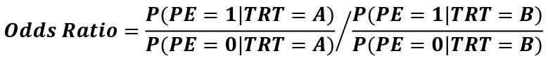
Statisticians really like odds ratios because they translate really nicely to logistic regressions.
Statistical Analysis of Randomized Controlled Trials (RCT)
- Define outcome <- Statistical Analysis plan/protocol
- Binary, continuous, etc.
- State the null hypothesis
- One or two sided; alpha level
- Descriptive statistics <- Data Analysis
- Determine appropriate statistical test
- Parameter estimates, confidence interval, p-value
- Write conclusions
Superiority Trial - We expect that the new treatment is better than the control
H0: μA = μB
HA: μA != μB
Note that we test the hypothesis two sided even though we think the effect will be one-directional. This is an FDA recommendation, one sided tests are allowed but use .025 level of significance. Two sided tests require larger samples size than one sided at alpha level .05.
Writing Conclusions
Statistical Methodology Section
- The primary outcome being tested
- Describe tests used, assumptions, and groups tested
Reporting of Results
- Mean and confidence intervals
- Test statistic values
- Reject or accept the null hypothesis
SAS
Generally we only need to specify a single test, but each test has its own assumptions
Parametric Tests
Parametric tests require the assumption of independence, equal variance and normality. When these assumptions do not hold, try either transformation or non-parametric tests.
We can get the same information from all the following procedures, but there are different options and defaults for each method
PROC TTEST, PROC GLM, PROC REG, PROC ANOVA
PROC TTEST
Test difference between means, and differences in variances via an F-Test
proc ttest data=dbp;
    class trt;
    var diff;
run;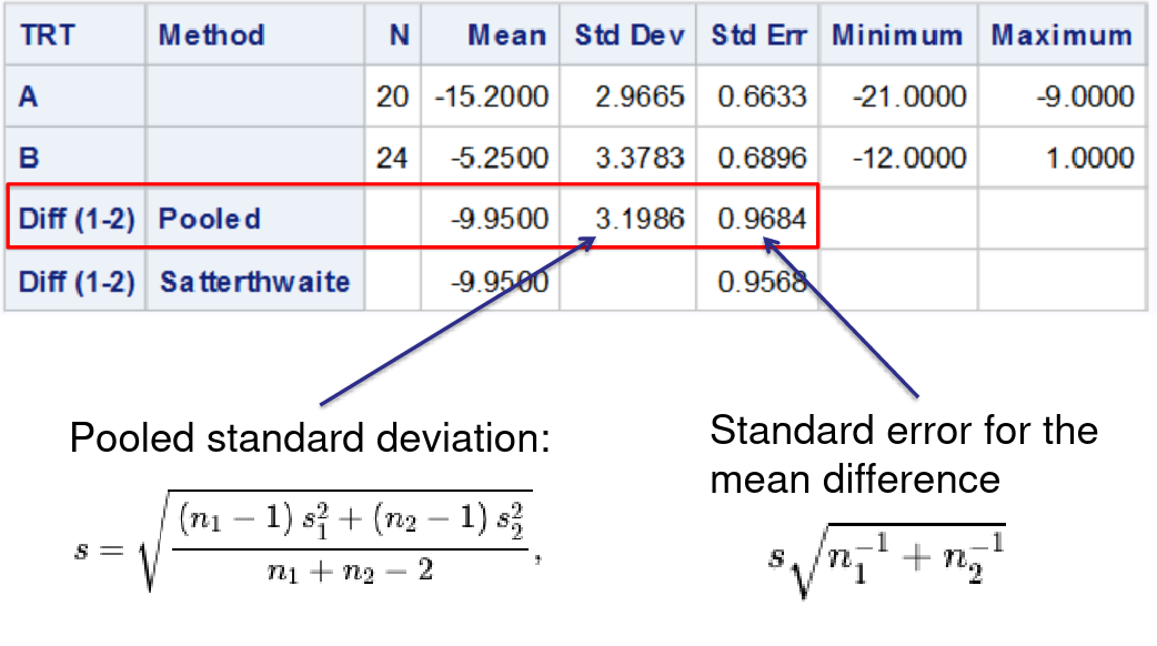
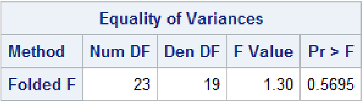
Welch's T-Test can be used if treatment groups have different variance
Proc Reg
Note, when using PROC REG or GLM always put a quit statement at the end or SAS will run forever.
Below we create a dummy variable for the treatment type.
data dbp;
	set dbp;
	if trt='A' then x=1;
	else x=0;
run;
proc reg data=dbp;
	model diff = x;
run; quit;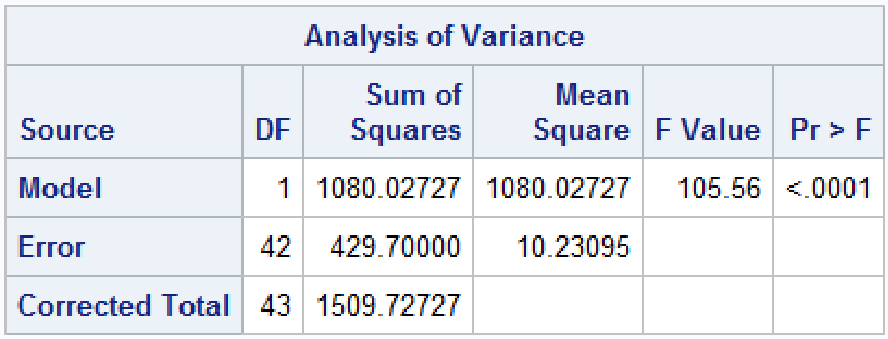
The F statistic is exactly the same p-value and square of the t-test under the assumption of equal variances
Proc GLM
Almost the same as PROC REG but no need for dummy variables
proc glm data=dbp;
	class trt;
	model diff=TRT /solution clparm;
	means TRT/hovtest=levene welch;
run;quit;
Non-Parametric Tests for Two Groups
Non-parametric groups only pay a very small penalty, if the data is normally distributed the test is ~95% as powerful as a ttest
Non-parametric Tests
PROC NPAR1WAY, PROC SURVEYSELECT
Wilcoxon Rank-Sum Test
Works very well on skewed data
proc npar1way data=dbp wilcoxon;
	class TRT;
	var diff;
	*exact wilcoxon; /* request for exact p-value - may take a while */
run;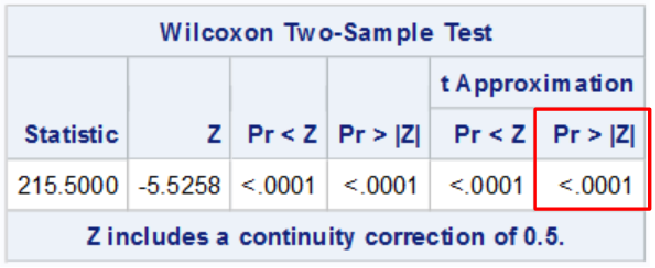
The highlighted is the two sided z test typically reported
Transforming Data
Natural logarithmic transformations are the most widely used in health data, where data often follows a log-normal distribution. Can only be used with positive values.
Running a t-test may not lead to an equivalent null hypothesis if the variances of the two groups are different
data dbp;
	set dbp;
	logAge=log(Age);
run;
proc univariate
	data=dbp;
	class TRT;
	histogram;
	var Age logAge;
run;
Bootstrap Confidence Intervals
How they work:
- Compute statistics of interest for the original data
- Resample B times from the data with replacement to form B bootstrap samples
- Compute statistics of interest on each bootstrap sample
- this creates the bootstrap distribution which approximates the sampling distribution
- Use the bootstrap distribution to obtain estimates such as confidence interval and standard error
/* 1. Compute statistics in the original data */
proc means data=new;
class trt;
var diff;
run;
/* 2. Bootstrap resampling */
proc surveyselect data=new noprint seed=1
out=BootSSFreq(rename=(Replicate=B))
method=urs /* resample with replacement */
samprate=1 /* each bootstrap sample has N observations */
/* OUTHITS */ /* option to suppress the frequency var */
reps=1000; /* generate 1000 bootstrap resamples */
run;
/* 3. Compute mean for each TRT group and bootstrap sample */
proc means data=BootSSFreq noprint;
class TRT;
by B;
freq NumberHits;
var diff;
output out=OutStats; /* approx sampling distribution */
run;
/* 4. Bootstrap distribution and confidence interval */
data boot_mean (keep=B diff TRT);
set OutStats ;
where _STAT_='MEAN' and _TYPE_=1;
run;
proc univariate data=boot_mean noprint;
class TRT;
histogram;
var diff;
output out=boot_ci pctlpre=boot_95CI_ pctlpts=2.5 97.5
pctlname=Lower Upper;
run;
proc print data=boot_ci noobs;
title "Bootstrap confidence intervals";
run; title;
Baseline Variable Adjustment
Baseline covariates are variables expected to influence the outcome, measured before the start of the intervention. They should describe the population enrolled in the study (Table 1 in all RCT papers). We need to decide what variables to measure, if the groups are comparable, and analyze the interactions and possible confounders.
Post-Randomization variables are collected after randomization. For the purpose of estimating treatment effect we never adjust for post-randomization covariates. Post-randomization variables are crucial for er-protocol effect estimation, mediation, and certain types of trials with adaptive design.
Adjusting for Baseline Imbalance
Conditional Methods included regression models, stratification, propensity score, etc.
Marginal Methods inverse probability weighting, standardization, double robust estimation, etc.
So we know randomization around averages produces balance between groups with respect to all measured and unmeasured factors that may influence outcome. However, this does not guarantee balance in any specific trial for any specific variable. Imbalance is common in trials with small sample size, the rule of thumb is the likelihood of baseline is small when n > 200.
If the treatment groups differ in baseline characteristics any difference in the outcome between group might be due to the difference in characteristics.
The best place to address baseline imbalance is in the design stage by creating a proper randomization strategy. In modern statistics, we can also adjust baseline covariates during the analysis stage.
Assessing Imbalance
Identify covariates expected to have an important influence on the primary outcome and specify how to account for them in the analysis in order to improve precision and to compensate for lack of balance between groups.
Statistical testing is controversial for multiple reasons: multiple testing, its hard to reject the null in small trials and the philosophical problem of type I & II errors. However, the p-value can be adjusted to identify imbalances in baseline by choosing a larger cut-off. There is additional controversy over whether to include p-value in "Table 1".
Stratification can sometimes be used to adjust for factors to improve precision of the treatment effect estimate.
We can assess imbalance through ANOVA output from proc glm in sas:
proc glm data=myzinc;
class zinc (ref='0') female (ref='0') heavy (ref='0') ;
where month=18;
model score_v=zinc female heavy/solution clparm;
run;quit;
The F-test of the model in the output is a test that any one of the predictors is significantly associated with the outcome (not very useful)
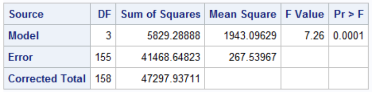
F = MS_model / MS_error
In the sum of squares table we can test whether adding new variables improves model fit:
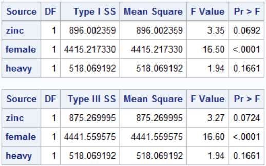
Note that Type I Sum of Squares is cumulative SS if we added the predictors from top to bottom. In Type III sum of sqaures every predictor is adjusted for every other predictor, it is much more widely used.
Analysis of Covariance (ANCOVA)
When an outcome is continuous, adjusting for a baseline covariate that is correlated with the primary outcome can improve precision of treatment effect estimates. Differences between outcome values which can be attributed to differences in the baseline covariate can be removed, leading to more precise estimates.
- The amount of precision gained depends on the strength of the correlation
- Adjusting for variables that are not correlated with the outcome will decrease precision
- Modeling the outcome at the end of the study should be equivalent to the change in outcome between the study end and baseline
proc glm data=myzinc;
class zinc (ref='0') female (ref='0') heavy (ref='0') ;
where month=18;
model score_v=zinc score_v_0 female heavy/solution
clparm;
run;quit;
Binary Outcomes
Instead of average treatment effect we can define a binary variable and use a logistic function to get the odds ratio and other magnitude of effect measures. If the covariate is strongly correlated with outcome then this adjustment will usually lose precision.
data myzinc;
set myzinc;
lower_score=0;
if score_v<score_v_0 then lower_score=1;
run;

proc logistic data=myzinc;
where month=18;
class zinc (ref='0') female (ref='0') heavy (ref='0') ;
model lower_score(event='1')=zinc female heavy /risklimits;
run;
Inverse Probability Weighting (IPW)
- Each individual receives a weight equal to the inverse (reciprocal) of the probability of being assigned to the treatment they received conditional on their baseline covariates L.
Wi = 1 / P(A=a | L) - Fit an adjusted model in the weighted population
- This final model is not conditional on L
- Adjustment for baseline covariates is achieved through weighting where the weights are computed in step 1
- Confidence intervals must be based on robust or bootstrap standard error
*** Step 1: Compute the propensity score (ie
* probability of treatment assignment conditional
* on baseline covariates);
proc logistic data = myzinc;
ods exclude ClassLevelInfo ModelAnova
Association FitStatistics GlobalTests;
class female (ref='0') heavy (ref='0') ;
where month=18;
model zinc(event='1') = female heavy
score_v_0 ;
output out=est_prob p=p_zinc;
run;quit;

*** Step 2: Compute inverse probability weights;
data est_prob;
set est_prob;
if zinc=1 then wt= 1/p_zinc;
else if zinc=0 then wt= 1/(1-p_zinc);

*** Step 3: estimate treatment effect in the weighted
population;
proc genmod data=est_prob;
class id;
weight wt;
model score_v= zinc;
estimate ‘Zinc' intercept 1 zinc 1;
estimate 'Placebo' intercept 1 zinc 0;
repeated subject=id / type=ind;
run;quit;
Disadvantages:
- Relies on assumption of correct model specification
- Typically less efficient than regression adjustment and leads to wider confidence intervals
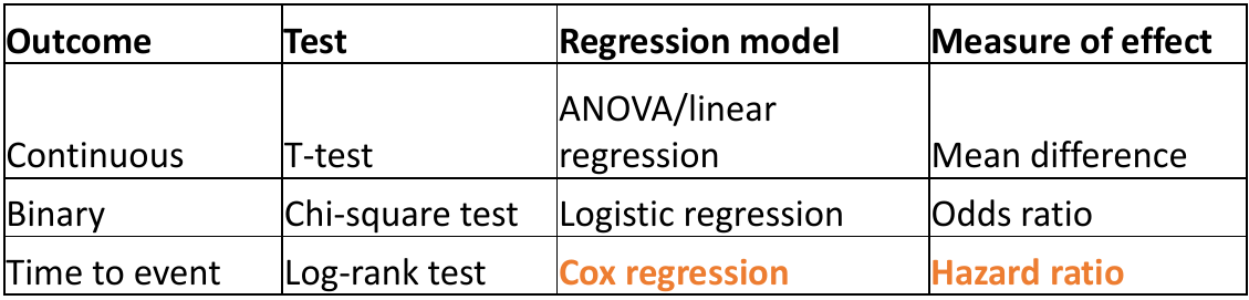
Survival Analysis in Clinical Trials
We've already covered survival analysis in great detail here. This will be review, application to clinical trials, and SAS implementation.
Survival analysis uses class methods of studying occurrence and time of events; it was traditionally designed to study death, but can be used with any type of time to event outcome. These are special cases when a t-test is not appropriate; as the data is skewed and there are values that need to be censored before the end of study.
Participants enter the study event-free and the outcome is to assess if and when the event occurred. We can then investigate if the event occurs differently in other groups. Patients are typically randomized at different dates in the recruitment period and time is measured on a continuous scale. We measure time in the study as the time between randomization and either the patient:
- Has the event (Failure time)
- Is last measured in the study and does not have the event (Censoring time)
Right Censoring
Most common form of censoring and the ideal scenario; Participants are followed for a time but the event of interest does not occur. All we know is that the time of the event is greater than a certain value but it is unknown by how much.
- End of study
- Loss to follow-up (withdrawal or dis-enrollment)
- A completing risk - A different event that occurs and makes it impossible to determine when the event of interest occurs
Interval Censoring
The time for an event occurs between two time points in the study but the investigators do not know the exact date. This could occur when the outcome is self-reported at 3 month intervals, for example. There are special methods for interval censoring in SAS we will not cover here (PROC ICLIFETEST)
The Survival Function
The survival function S(t) is a mathematical function that represents the probability of surviving beyond a particular time t. We can plot the % surviving (without event) on the Y-axis and time on the X-axis to see when most of the events occurred.
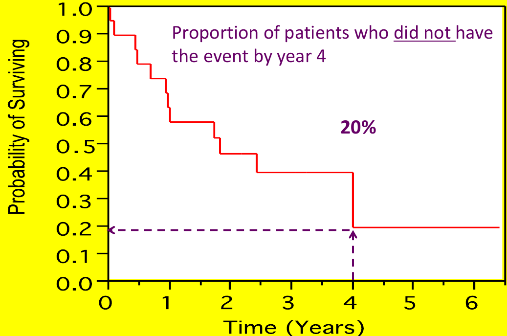
Each step is an "event", but cesnroing events are often marked as an 'X' (no step)
The most commonly used method for estimation of the survival function is the Kaplan-Meier (or product-limit estimator). Suppose there are k distinct event times and n subjects at risk of event, with dj subjects with outcome at time tj: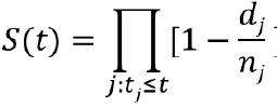
We can visualize this in a chart: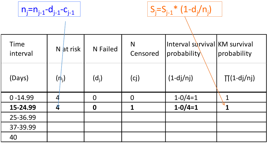
Kaplan-Meier estimates are calculated from the conditional probability of experiencing the event
P(A, B, C) = P(C | A, B)*P(B|A)*P(A)
Ex. S(37) -> Survival estimate at day 37 = P(T > 37 & T > 25 & T > 15) -> Probability of surviving past day 37, 25 and 15
* Computes tables of survival estimates, KM survival curves and log-rank test;
proc lifetest data=mysurv;
time time*cvd_death(0);
strata treat;
run;
Above cvd_death is the name of the event/censoring variable, and the strata is what we want to compare survival. 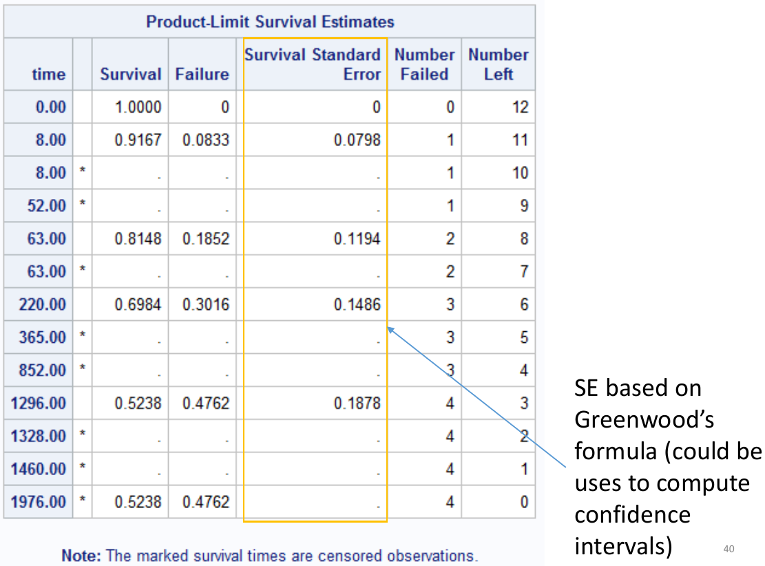
In the above sample output:
- "Survival" Represents the KM survival estimate
- "Failure" is the cumulative probability of the event (1 - KM probability).
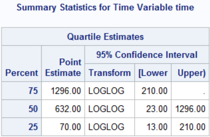
The quartile estimates Point Estimate gives the smallest event time such that the probability of event is greater than [.25/.5/.75]. There may not be a point estimate if the number of observed events/Failure never reached the percent.
Comparing Survival Curves
Are the curves similar? At what point do they diverge? When do most events occur?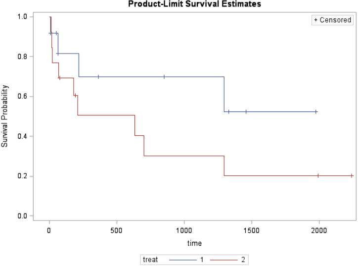
H0: No difference in survival between treatments (KM survival curves are the same)
HA: Difference in survival between treatments (KM survival curves are the different)
![]()
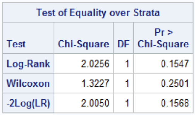
Where r is the number of event times d1j is the number of events in group 1 at time j and eij is the expected number of events in group 1 at time j.
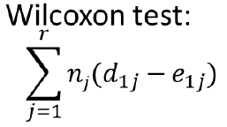
Where nj is number of individuals at risk at each time point (Weighted sum); Gives more weight to early times than later times
Both log-rank and Wilcoxon test follow a chi-square distribution with 1 df (if G treatments then df = G - 1)
Assumption: Non-Informative Censoring
We assume all individuals who are censored have the same risk of the event (or prognosis) as those who remain in the study (conditional on explanatory variables). There is no statistical test for informative censoring, we just need to adjust estimates for variables that are likely to affect the rate of censoring (need regression models).
Ex. The outcome is death and very sick subjects are less likely to attend study visits.
Comparing Treatments
The Hazard (or hazard rate) is the instantaneous risk/rate of experiencing the event at time t. It is not a risk.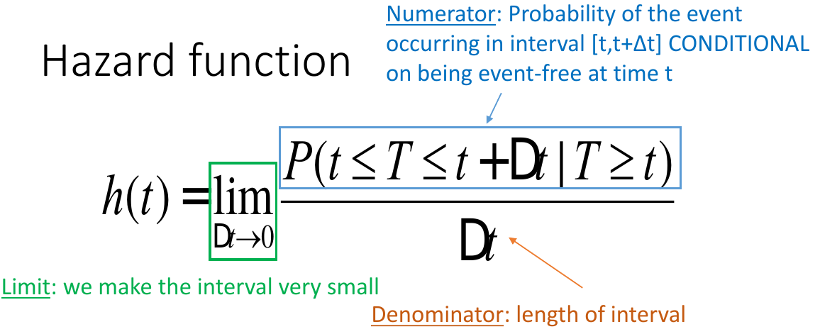
Interpretation: "The hazard of event for the new treatment is 44% of the hazard of the active control group. The 95% CI contains 1 so it is not significant."
In the Cox Proportional Hazards Regression we create dummy variables fro the treatment group: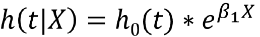
Which can be expressed as:![]()
HR<1 (or β<0): lower hazard of the event compared to reference group
HR>1 (or β>0): larger hazard of the event compared to reference group
Proportional Hazards assumption must be met for a Cox model. That is the separate treatment plots of ln(-ln(S(t)) vs t should be parallel.
Also we can adjust for covariates just like in proc glm ANOVA where we assess interaction and factors.
*Cox Model;
proc phreg data=mysurv;
class treat (param=ref ref='2');
model time*cvd_death(0)=
treat/risklimits;
run;

*Log-log survival plot;
proc lifetest data=mysurv plots=(loglogs);
time time*cvdmort(0);
strata treat;
run;
Partial Likelihood
The LR function for Cox models can be factored into
- One part that depends on h0t and β
- The other part that depends on β alone (partial likelihood)
- We treat the partial likelihood as an ordinary likelihood:
• Estimate values of β that maximize partial likelihood
• Asymptotically consistent and normally distributed
• Estimates are (only slightly) less efficient
Multiple Comparisons
There are some situations where it may be necessary to have multiple hypothesis tests; ANOVA with more than 2 tables, genetic data, interim analysis, multiple outcomes, etc. Often times clinical trials may have 3 or more arms to reduce administrative burden and improve efficiency and comparability.
Recall hypothesis tests are a way to determine the truth about 2 states and 2 possible outcomes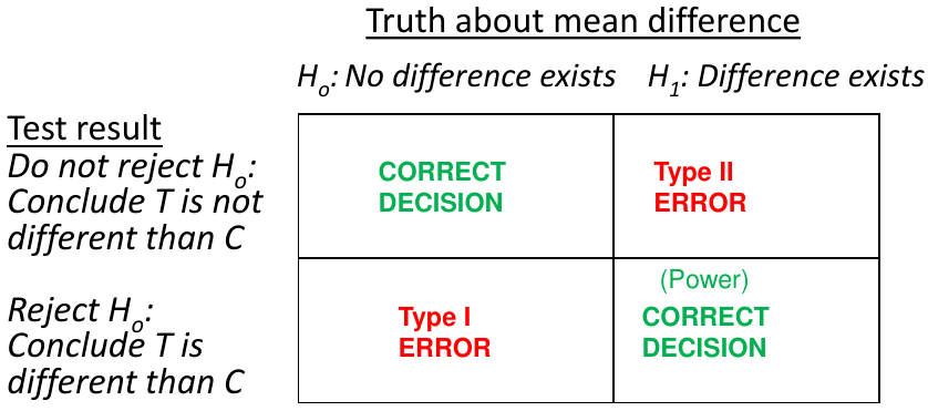
α = probability of a Type 1 error; β = probability of a Type 2 error; 1 - β = power
Assume we carry out m independent statistical tests with significance level α, this means the probability of not making a Type 1 error in any test is: (1-α)*(1-α)*(1-α)*...*(1-α)=(1-α)m
Multiplicity may occur when we use more complex designs, such as 3 or more treatment groups, multiple outcomes, or repeated measurements on the same outcome.
Types of Error Rates
- Comparison-wise Error Rate (CER)
- Type 1 error rate for each comparison
- Family-wise (FWER) or experiment-wise error rate
- Type 1 error rate for the entire group of comparisons
Analytic Strategies
- Define success as "all-or-nothing"
- All tests must be significant
- Ex. Back to Health study where there were two endpoints (a questionnaire and a visual analog scale of pain) the study was only a success when both endpoints showed that yoga was non-inferior to physical therapy for chronic lower back pain.
- This method does not inflate the FWER
- Define success as "either-or" and adjust for multiplicity
- At least one test is significant
- Ex. A burn treatment that could speed up healing or reduce scarring but we are not sure which.
- If both nulls are true the FWER is inflated can be ~ .1
- Use a composite endpoint
- Combining multiple clinical outcomes into a single variable
- Only one test to perform
- No inflation of the FWER
Adjusting for Multiplicity
- Single Step Procedures
- Test each null hypothesis independently of the other hypotheses, order is not important.
- Bonferroni, Tukey, Dunnett
- Stepwise procedures
- Testing is done is a sequence
- Data-driven ordering - The testing sequence is not specified at proir and the hypotheses are tested in order of significance/p-value
- Pre-specified hypothesis ordering - The hypotheses are tested in a pre-specified order
- Holm, Fixed-sequence
- Other multiple comparison procedures:
- Fisher's Least Significant Differences (LSD) - no alpha adjustment
Fisher's Least Significant Differences
We complete the global ANOVA first, if it rejected we simply complete the pairwise comparisons and do not correct the p-values. Easiest method, but this requires the global ANOVA is rejected. The FWER is only controlled when all null hypotheses are true.
proc glm data=headache;
class group;
model outcome=group;
lsmeans group / tdiff pdiff stderr cl;
* tdiff = t-statistics and p-values for pairwise tests;
* pdiff = p-values for pairwise tests;
* stderr = standard errors for means;
* cl = confidence limits;
run;quit;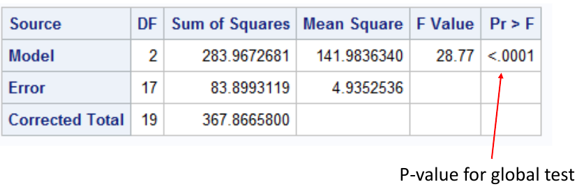
This output suggests we reject the null hypothesis and conclude the mean is different in at least one group. Thus we can do the rest of the pairwise comparisons: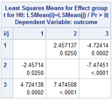
P-Value (Single Step) Adjustments
To correct the comparison-wise alpha level to allow the family-wise comparison level to be controlled at .05. For example, there are two ways to implement the Bonferroni correction:
- Divide the comparison-wise alpha level by the number of comparison and use that as the threshold
- Multiply the observed p-values by the number of comparisons and compare to .05
* Bonferroni correction;
proc glm data=headache;
class group;
model outcome=group;
lsmeans group / tdiff pdiff stderr cl adjust=bon;
run;
quit;

* We can also use Bonferroni correction
with a control group;
proc glm data=headache;
class group;
model outcome=group;
lsmeans group / tdiff
pdiff=control(‘Placebo’) stderr cl
adjust=bon;
run;
quit;

* Tukey-Kramer correction;
proc glm data=headache;
class group;
model outcome=group;
lsmeans group / tdiff pdiff stderr cl adjust=tukey;
run;
quit;

* Dunnett;
proc glm data=headache;
class group;
model outcome=group;
lsmeans group / tdiff
pdiff=control(‘Placebo’) stderr cl
adjust=dunnett;
run;
quit;
The Dunnett's test takes advantage of correlations among test statistics, generally less conservative than Bonferroni (lower Type 2 error rate).
Step-Wise Adjustments
- Holm step-down algorithm (AKA "Stepdown Bonferroni")
- Rank the P-values from smallest to largest along with the null hypotheses
- Step 1: Reject H0_1 if p1 <= α/m, if its rejected go to step 2 otherwise stop and do not reject any further hypotheses.
- Step i = 2, ..., m-1: Reject H0_i if pi <= α/(m-i+1). If H0_i is rejected go to step i + 1 otherwise stop and do not reject any remaining hypotheses
- Step m: Reject H0_m if pm <= α
data pvals;
input test $ raw_p @@;
cards;
AvP 0.0002 NvP 0.0001 NvA 0.025
run;
proc multtest pdata=pvals bonferroni holm out=adjp;
run;- Fixed-sequence procedure
- Suppose there is a natural ordering of the null hypotheses (such as clinical importance) fixed in advance
- The fixed-sequence procedure performs the tests in order without an adjustment for multiplicity as long as all the preceding tests had significant results
- It's the same process as above, do not reject any remaining hypotheses once H0_j is rejected
The FWER is controlled because a hypothesis is tested conditionally on having rejected all the hypotheses that came previously.
Non-Inferiority in Clinical Trials
Usually clinical trials should show if a new treatment is superior to placebo or no treatment, but as we've previously discussed it is not always ethical to give out a placebo when an effective treatment has been identified.
The goal of non-inferiority trials is to to demonstrate a new treatment (T) is NOT inferior (no worse than) the best available treatment (C), given the effect of the active control (compared to placebo or no treatment) has already been established.
Non-Inferior = Not Unacceptably Worse
In practice non-inferiority trials assess:
- If T is not necessarily more efficacious (superior) than C
- If T could be not as effective as C, but could have potential ancillary benefits:
- Lower procedural risks (safety)
- Less side effects
- Improved convenience
- Favorable costs
- Non-inferiority margin: How much worse we are willing to accept T compared with C
Hypothesis Testing
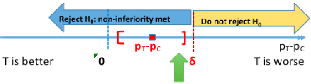
H0: πT - πC <= -δ (inferior)
HA: πT - πC > -δ (non-inferior)
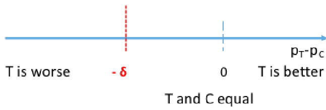
π represents the population level experimental and control proportions/risk of outcome
δ is the non-inferiority margin
Rejecting the null means non-inferiority is met, failing to reject the null means the new treatment is inferior. Both non-inferiority and superiority are met if T falls above the 'T and C' are equal point.
The null can also be rewritten as πT + δ <= πC, but SAS uses: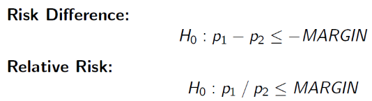
Because these settings cannot be changed, consider your margin carefully
Computing the 95% confidence interval for the difference in πT - πC we would reject the null when the CI's lower boundary is greater than -δ.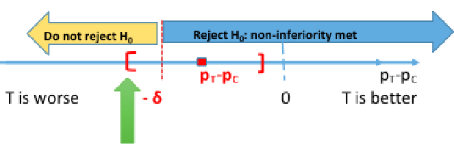
This is because we are only computing a one-sided test. Note that SAS gives us both sides of the confidence interval, so it is important to know which side is being tested.
Binary Outcomes - Farrington-Manning Test
Below is a Z test statistic following a normal approximation to the binomial distribution: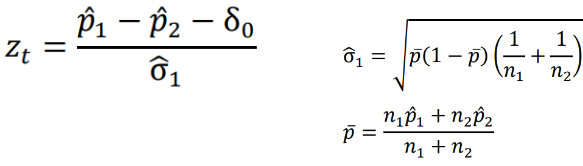
The Farrington-Manning Test (used in SAS) uses restricted maximum likelihood estimation to estimate variance of risk difference or risk ratio under non-inferiority null: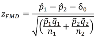
Also note the the FDA requirement for non-inferiority is alpha=.025.
In the SAS sample code below we test the positive outcome of HVC treatment, testing a margin of .105:
data hepatitis;
input trt outcome count;
cards;
24 0 13
24 1 149
48 0 20
48 1 140
;
run;

*Positive Outcome;
proc freq data=hepatitis;
table trt*outcome/riskdiff(column=2 noninf method=fm margin=0.105) alpha=0.025;
weight count;
run;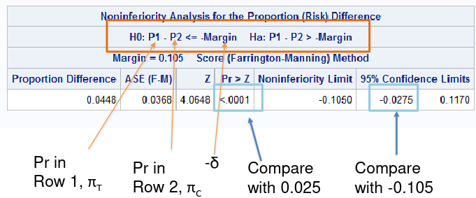
In a negative outcome, where we are testing if something is made worse, we would look at the upper boundary of the confidence interval compared to -δ.
So far we've been testing the risk difference, but we may want to test the relative risk (AKA risk ratio) of outcome. Then our null hypothesis would look like: H0: πT / πC >= R
Keep in mind when considering risk ratio or risk difference:
For a negative outcome:
- It takes a larger sample to prove non-inferiority using the RR approach than absolute RD approach
- A sample size yielding power of 80% with risk difference only yields about 70% power with RR approach
For a positive outcome:
- It takes a larger sample to prove non-inferiority using the RD approach than RR
*Sample Size - Risk Difference;
proc power;
twosamplefreq alpha=0.025
groupproportions = (0.30, 0.30)
test=fm
sides=1
power=0.80
nullproportiondiff = 0.10 0.20
npergroup=.;
run;

*Sample Size - Risk Ratio;
proc power;
twosamplefreq alpha=0.025
groupproportions = (0.30, 0.30)
test=fm_rr
sides=1
power=0.80
nullrelativerisk = 1.67 1.33
npergroup=.
;
run;
Choice of Inferiority Margin
The trial should have the ability to recognize when the new drug T is not inferior to the active control C and superior to the placebo P by a specified amount.
The two-step procedure proposed by the FDA Guidance on Non-Inferiority trials (updated 2016), for a risk difference approach:
- Define M1: Effect of active control relative to placebo (πT - πC or its best estimate)
- M1 is the smallest (most conservative) estimate of C against P
- M1 must be > 0, otherwise there is no evidence that C is superior to P
- Average/combine placebo minus control RD from previous placebo vs the control trial (e.g. via meta-analysis)
- Define M2: The non-inferiority margin is HALF of M1
- M2 is the largest clinically acceptable difference (degree of inferiority) of the test drug compared to the active control
- Should be set as <= .5*M1
Issues in Non-Inferiority Trials
There are several challenges with non-inferiority trials for investigators and regulatory bodies:
- Assay sensitivity
- A trial that demonstrates non-inferiority does not demonstrate efficacy
- Both C and T could be similarly ineffective
- In non-inferiority trials we make an (untestable) assumption that the control treatment is effective (assay sensitivity) in the trial setting
- Factors that may induce assay insensitivity: lower event rates, poor adherence, new concomitant medications, etc. compared to the placebo-controlled trials
- A related concept is assay constancy: the treatment effect of C s no treatment P is the same as in the trials which informed the choice of margin
- A trial that demonstrates non-inferiority does not demonstrate efficacy
- Less incentives to reduce errors
- Factors that reduce the difference between treatments (measurement error, low event rates, adherence, etc) will increase the likelihood of declaring non-inferiority (success)
- Unlikely in superiority trials, bias toward the null improves the chance of trial success
- Efficacy creep
- Efficacy creep or biocreep can occur when a slightly inferior treatment becomes the new standard of care for the next gen non-inferiority trials
- If it happens repeatedly we end up with a standard of care no better than the placebo
- Degradation of the true efficacy of the comparative drug
- Ideally a control treatment C should have been previously known to be effective against placebo P directly
- Primary approach to analysis (ITT or PP)
- Intention to treat (ITT) is often considered the primary approach to analysis, but ITT is known to make groups appear more similar mostly due to including subject who are non-compliant
- Per-protocol (PP) can make groups appear more similar or more different
- If we use PP instead we lose benefits of randomization (by removing non-compliant participants)
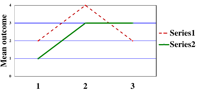
Effect Modification and Interaction
Interaction is when a treatment effect is different across different subgroups of the population defined by a baseline covariate. Commonly examined effect modifiers include: demographic variables, study location, or baseline prognostic factors.
If an interaction does exist:
- We may not be able to provide a single summary measure
- A treatment may be beneficial to some subgroups but harmful to others
- We may need to conduce subgroup analyses to identify the treatment effect within each subgroup.
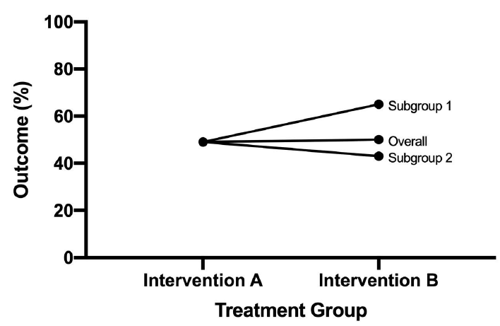
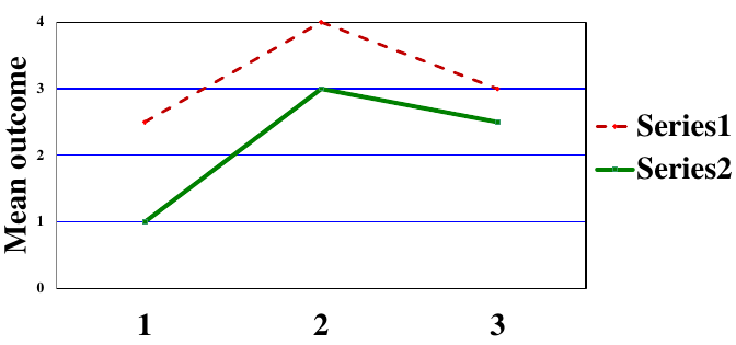
Types of Statistical Interactions
- Quantitative: Direction of the effect of an exposure on an outcome is the same for different subgroups but the size of the effects differs

- Qualitative: Direction of the effect of an exposure on an outcome differs for different subgroups

A potential issue that arises with assessing interaction is that the sample size within a subgroup will be smaller than for the whole trial population and there will be less power to detect an effect. To account for this we can adjust the sample size requirement for interactions of interest, or define a limited number of pre-specified exploratory subgroup analyses (multiple testing needs to be accounted for).
Statistical Assessment of Interaction
Interaction F is testing:
H0: No interaction vs H1: Interaction
*Adjusted Treatment Comparison;
proc glm;
class trt sex;
model change=trt sex/solution clparm;
run;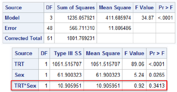
The FDA rule is to assess interactions at .15 level of significance. This is conservative and circumvents low power issues; If the interaction exists it may have a relatively low probability of obtaining a significant interaction result.
Other options:
- Cochran-Mantel-Hansel approach (PROC FREQ)
- Include CMH option in table statement
- Provides 3 types of info:
- Test for interaction by center (Breslow-Day Homogeneity Test)
- The Breslow-Day Test of Interaction tests the null hypothesis that odds ratios across q strata are all equal; Under the null the statistic has a chi-square distribution with q-1 df (strata-1)
- BD test requires large sample size within each stratum
- At least 80% of the expected cell counts should be > 5
- Tarone's modification has slightly more accurate p-values when values are small
- (add bdt to table options)
- Summary measures of association (weighted average of stratum specific OR or RR)
- Test for treatment effect adjusting for center
- Test for interaction by center (Breslow-Day Homogeneity Test)
- Logistic Regression (PROC LOGISTIC)
- Include the interaction term(s) in the model statement
*Cochran-Mantel-Haenszel Approach;
proc freq;
*Order: Factor*Treatment*Outcome;
table center*arm*corabn/cmh;
weight count;
run;

* Assessing treatment-by-center interaction with logistic regression;
proc logistic data=kawasaki;
class arm(param=ref ref='2-ASA') center;
model corabn(event='ABNORMAL')=arm|center /rl;
freq count;
oddsratio arm / at (center=all);
run;
Interpretation
If the interaction is qualitative it would be meaningless to talk about an "overall" treatment difference. We would need to investigate the cause of interaction and if it invalidates the study through subgroup analysis.
If non-significant or quantitative we can "ignore" interaction (remove from model assessing treatment effect)
When an interaction term is present, the main effects alone cannot be interpreted without being relative to the state of other variables.
Dummy Variable Approach to Interaction
![]()
In SAS we represent interaction in a regression model using binary variables.
*Code Binary Variable;
data dbp;
set dbp;
*Dummy variables;
if sex='F' then new_sex=1;
else new_sex=0;
if trt='A' then new_trt=1;
else new_trt=0;
*Interaction term(s);
trt_sex=new_trt*new_sex;
run;

*Model with interaction;
proc reg data=dbp;
model change=new_trt new_sex trt_sex;
*Test for interaction;
INTERACTION: test trt_sex=0;
run;
Interim Analysis and Data Monitoring
Clinical trials are often longitudinal in nature. It is often impossible to enroll all subjects at the same time, so it can take a long time to complete a longitudinal study. Over the course of the trial one needs to consider administrative monitoring, safety monitoring and efficacy monitoring.
Efficacy monitoring can be performed by taking interim looks at the primary endpoint data (prior to all subjects being enrolled or all subjects completing treatment). This is because:
- It potentially stops the trial early if there is convincing evidence of benefit or harm of the new product
- It potentially stops the trial for futility, in other words the chance of significant beneficial effect by the end of the study is small given observed data
- Re-estimate final sample size required to yield adequate power to obtain a significant result
Interim analysis evaluates for early efficacy, early futility, safety concerns, or adaptive design with respect to sample size or power.
Group Sequential Design
A common type of study design for interim analysis is GSD, in which data are analyzed at regular intervals.
- Determine a priori the number of interim "looks"
- Let K = # of total planned analyses including final (K >= 2)
- For simplicity, assume 2 groups and that subjects are randomized in a 1:1 manner
- After every n = N/K subjects are enrolled and followed for a specific time period, perform an interim analysis on all subjects followed cumulatively
- If there is a significant treatment difference at any point, consider stopping the study
Due to multiple testing the probability of observing at least one significant interim result is much greater than the overall α = .05, as a result the interim analyses should NOT be performed using the family-wise error rate. The data at each interim analysis contains data from the previous interim and thus are not independent.
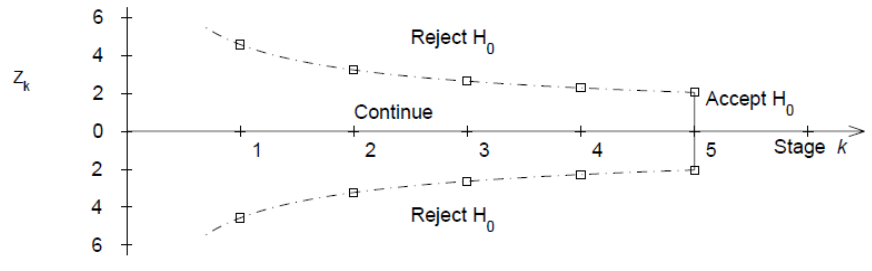
Equivalently we would have K critical values for each interim:
- First interim analysis compare test statistic to critical value Z1 |> c1. If significant then stop the trial.
- Second interim analysis compare test statistic to critical value Z2 |> c2. If significant stop the trial
- ...
- Final analysis compare test statistic to critical value Xk |> ck.
Pocock Approach (1977)
Derives constant critical values across all stages to maintain the overall significance level at .05. The critical value depends on the number of interim analyses, but is the same for each interim look.
Ex. When K=5, Z critical value = 2.413 for each interim and the final analysis. When K=4, Z critical value = 2.361.
O'Brien-Fleming Approach (1979)
Proposed sequential testing procedure that has critical values (in absolute value) decrease over the stages. Z critical value depends on total number of interim analyses and the stage of the interim analysis. The critical Z value depends on the total number of interim analyses and the stage of the interim analysis.
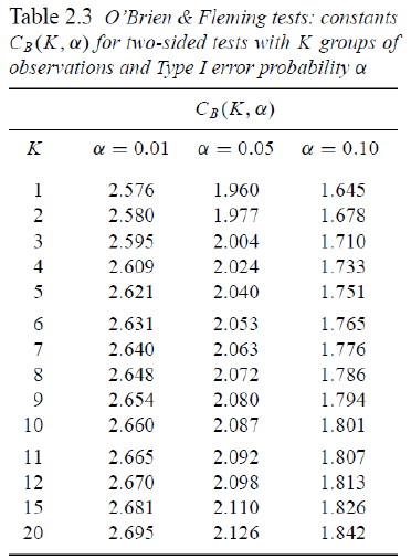
Ex. For K = 5 after after 200 subjects completed:
- C5 = 2.040 a constant determined by O'Brien-Fleming)
- First look critical value is: sqrt(5/1)*2.04 = 4.56
- Second look critical value: sqrt(5/2)*2.04 = 3.23
- ...
- Critical value final look: sqrt(5/5)*2.04 = 2.04
This makes it more difficult to declare superiority at "earlier" looks, but does lose much of the original alpha at the final look. This is more conservative than Pocock and the recommended approach by the FDA on their 2010 Guidance on Adaptive Designs.
Controlling the Overall Significance Level
Issues with group sequential procedures:
- Need to specify a priori for the number of planned interim analyses
- The timing of interim analyses is generally not exact calendar time but "information time" (i.e. based on sample size or number of events)
- Assumes interim analyses performed after every n subjects complete follow-up (or y events occur)
- Difficult to schedule formal review procedures for interim analyses after every n subjects (or y events); may want to allow more flexibility in scheduling
- So the main issue is: How do we allow for more flexibility for unscheduled interim analysis?
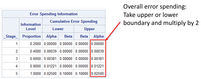
Alpha-Spending
From Lan and DeMets (1983) Biometrika: Adjust teh levels via an "alpha-spending function". Think of it like each analysis spends a bit of the alpha power.
- α(s) denotes alpha spending function.
- s = proportion of information (sample size or events) accrued
- s = 0 at the start of the study (0% information); α(0) = 0
- s = 1 is the end of the study (100% information); α(1) = 1
- α(sk) proportion of Type 1 error one is willing to spend up to time k
- Not a significance level
This can work in conjunction with O'Brien-Fleming.
Interpretation:
- If the first interim analysis occurs after 20% of information, reject treatment equality if p-value < .000001
- If the third interim analysis occurs after 60% of the subjects are in, reject treatment equality if p-value < .0074
Focus on the significance levels, note the the alpha spending and significance level are two distinct values and not equal. Computing critical values and corresponding significant levels require knowledge of multivariate distributions. There is no "simple" equation to get from α(s) to Z. Typically obtained via numerical integration.
/*
	plots=boundary - graph observed stanardized test statistics
    	at each interim
    errspend - give overall error spending
    bscale=pvalue - instead of critical values print p-values
    info=equal - equal intervals
    stop=reject - trying to reject the null (default)
*/
proc seqdesign errspend plots=boundary;
TwoSidedObrienFleming: design nstages=5 alpha=0.05
alt=twosided info=equal method=errfuncobf
stop=reject;
run;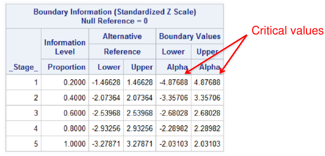
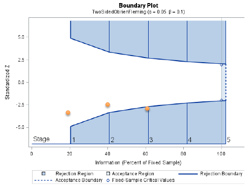
Notes that the bscale=pvalue option gives one tail of the distribution, so to get the significance level we need to multiply the upper or lower boundary by 2.
Pocock Approach in SAS
?* Pocock alpha-spending for a two-sided test with
	two-sided alpha spent of .05 by final analysis */
proc seqdesign errspend bscale=pvalue;
TwoSidedPocock: design nstages=5 alpha=0.05
alt=twosided info=equal method=poc stop=reject;
run;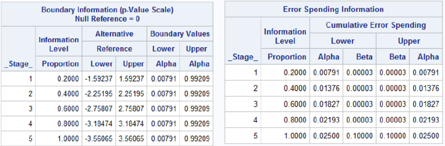
Interim Analyses For Safety
It is not necessarily easy from an administrative and study conduct perspective. We need to determine if data is still recent enough to be included. Weeks or months may pass between the last subject visit and generation of interim results due to data entry and cleaning. Depending on the size of the study, the ideal goal is to have a < 60-day lag between data collected at sites and the interim analysis report. Otherwise, interim analysis be be obsolete by the time analysis is completed.
Inspection of adverse events and serious adverse events is primary concern. Labs, vital signs, etc. need to be inspected. Unlike efficacy there is often no formal stopping rules based on p-values or a parametric test. If it is felt there is a safety concern, the study may be stopped regardless of significance between treatments.
The results of the interim analysis are also inspected by a Data Safety and Monitoring Board (DSMB), sometimes called the Data Monitoring Committee. Usually these consist of:
- >= 1 Statistician with expertise in interim analyses
- 2-4 clinicians with experience in the topic
- Maybe an ethicist (especially in government-sponsored trials)
- No member can be a study investigator
- DSMB is independent of the sponsor and all study activities
- DSMB can recommend to sponsor early stoppage when there is evidence of clear risk, harm or futility. But they cannot stop the trial themselves
The sponsor will often hire an outside group (Contract Research Organization or CRO) to perform the interim analyses. The statistician at CRO has a randomization schedule, and the analysis group cannot divulge ANY information to the sponsor or to any personnel involved in the study; It is presented to the independent Data Safety Monitoring Board.
Correlated Data in Clincal Trials
Note: My BS857 Notebook on Correlated Data goes much further in depth than the below.
So far we have focused on independent outcomes in clinical trials, but often times we work with correlated or non-independent outcomes in clinical trials; Such as crossover trials, repeated measurement designs or cluster randomized designs.
In a crossover trial each subject is used as its own control. Subjects are randomized to A then B or B then A. There is a "Wash-out" period used to avoid "carry-over" effect. It is best used for interventions whose effects can be measured after short period of administration. Carryover is the persistence of a treatment effecet applied in one period in a subsequent period of treatment.
The advantages of this design is there is no between-subject variability in statistical comparison; only within-subject variability. Since there is less variability we can use a smaller sample size.
The disadvantages are that there are very strict assumptions about carry-over effects. It is inappropriate for certain acute diseases, and doubles the duration of the study.
A simple analysis of a continuous outcome can be performed with a paired t-test. But to test if there is a carry-over effect we need to perform the treatment by period interaction.
In SAS, the PROC MIXED statement is used to account for correlated outcomes. The REPEATED statement tells SAS where the correlation occurs and how to handle it; Within the repeated statement time tells SAS what variable represents the repeated measurements, subject=id tells SAS what the clustering variable is, and type=un indicates a unstructured covariance matrix.
A covariance matrix is a collection of outcomes and variances at each time point and covariances and between outcomes at different points. Unstructured means that there are no restrictions placed on these values (all are estimated separately. There may be reasons to make simplifying assumptions.