# Modeling the Mean and Covariance
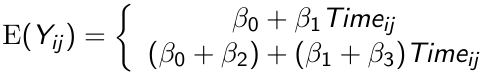
Suppose we have a model of mean response as a product of time on a continuous value:
[](https://bookstack.mitchellhenschel.com/uploads/images/gallery/2023-02/XsAimage.png)
The top is control and bottom is treatment. By allowing an index for the jth measurement we allow participants to have measurement in unequal time periods.
Consider the 3 hypotheses which could be tested:
- H0: β3 = 0 for testing parallelism between groups
- H0: β1 = 0 for testing flatness of change over time
- H0: β2 = 0 for testing differences between groups
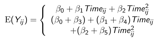
#### Quadratic Trends
Higher order terms should be tested (and removed from the model if appropriate) before the lower order terms
[](https://bookstack.mitchellhenschel.com/uploads/images/gallery/2023-02/TO5image.png)
In the above we would first test β2 = 0 and if this fails to be rejected we can remove the term and test β1 = 0
To avoid potential problems with collinearity we *center the variable of time around their mean before squaring it* in order to include it as a quadratic term
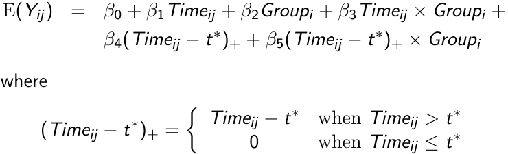
#### Linear Splines
There are application in which the mean response cannot be modeled accurately using a polynomial, like when the mean response increases rapidly for some duration and then more slowly thereafter. In such a case a linear spline model would be appropriate.
Assume the mean response follows a linear trend, **but the parameters change at a known time point t\***; We can write the following linear spline model with a **knot** at time t\*
[](https://bookstack.mitchellhenschel.com/uploads/images/gallery/2023-02/jhzimage.png)
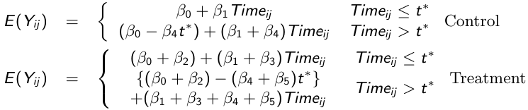
We can then write the model separately for each group before and after t\*
[](https://bookstack.mitchellhenschel.com/uploads/images/gallery/2023-02/jGHimage.png)
We can test the following hypotheses:
- H0: β3 = β5 = 0 for testing differences in patterns of change
- H0: β3 = 0 for testing group differences in patterns of change prior to t\*
- H0: β4 = β5 = 0 for testing changes in the linear trend model after t\*
##### Comparing Nested Models
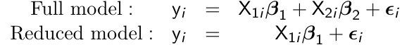
When comparing nested models with respect to mean response, we can compute a likeliood ratio test (LTR) by running an ML (not REML) under the two models; full and reduced.
For example:
[](https://bookstack.mitchellhenschel.com/uploads/images/gallery/2023-02/EMNimage.png)
testing for β2 = 0 is given by:
LTR = 2 (ℓ(β1, β2) - ℓ(β2))
For non-nested models we can use AIC or BIC:
AIC = -2(ℓ - c)
BIC = -2(ℓ - log(n)\*c)
Where ℓ is the maximized log-likelihood, c is the number of regression parameters and n is the number of subjects. Select the model that minimized AIC or BIC. The disadvantage of this method is they are empirically/evidence based and we cannot use them to perform any inference.
## Covariance Pattern Models
One of the most important aspects in modeling correlated data is estimating the covariance structure between measurement occasions. There is no single way of modeling the covariance structure, and a balance needs to be found when imposing structure.
- Too little structure may lead to many parameters for limited data, adversely effecting precision of β
- Too much structure improves β precision but increases the risk of mis-specification that could result in misleading inferences
##### Unstructured Covariance
For p measurement occasions:
[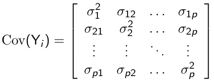](https://bookstack.mitchellhenschel.com/uploads/images/gallery/2023-02/iTpimage.png)
The covariance matrix must always be symmetric and positive-definite. The latter condition ensures that even though the repeated measurements can be highly correlated, none of them can be expressed as a linear combination of the others.
\+ No explicit structure required for the covariance among the repeated measures
\+ Can handle non-constant variance
\- Unstructured covariance has (p\*(p+1))/2 parameters. Even for a moderate number of repeated measurements the number of parameters needed to be estimated could be large
\- Requires all individuals have the same measurement occasions. No irregular intervals
##### Compound Symmetry
For p measurement occasions, the compound symmetry model has the following form:
[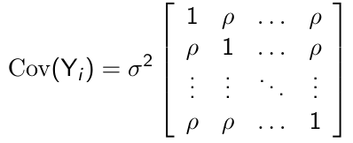](https://bookstack.mitchellhenschel.com/uploads/images/gallery/2023-02/pINimage.png)
\+ Very parsimonious, with only two parameters to be estimated regardless of the measurement occasions
\+ Very appealing for certain designs, such as cluster sampling
\- Requires strong assumption that the correlation between any pair of measurements to be the same no matter how large the time interval between the measurement is
\- Assumes constant variance over time
##### Heterogeneous Compound Symmetry
For p measurement occasions, the heterogeneous compound symmetry model has the following form
[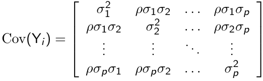](https://bookstack.mitchellhenschel.com/uploads/images/gallery/2023-02/WStimage.png)
This is a more flexible structure than CS, since it allows non-constant variance but with a smaller number of parameters to be estimated compared to unstructured covariance
##### First-Order Autoregressive Structure
For p measurement occasions the unstructured covariance has the following form:
[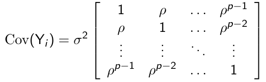](https://bookstack.mitchellhenschel.com/uploads/images/gallery/2023-02/1K9image.png)
\+ Very parsimonious, with only two parameters to be estimated regardless of the measurement occasions
\+ Appealing for longitudinal studies since the correlations decline over time as the distance between pairs of measurements increases
\- Requires all measurements to be made at equal intervals of time
\- Assumes constant variance over time
##### Heterogenous First-Order Autoregressive Structure
The constant variance assumption can be relaxed and we can have a heterogeneous AR(1) covariance pattern model:
[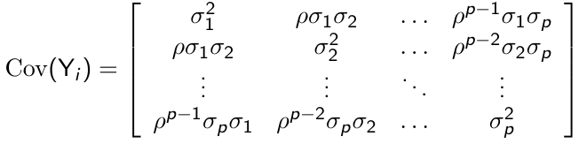](https://bookstack.mitchellhenschel.com/uploads/images/gallery/2023-02/gfNimage.png)
##### Exponential Structure
When measurements are not equally spaced over time the AR(1) covariance structure can be reformulated as an exponential structure. Let {ti1 ... tip} denote the observation time for subject i, and assume variance is constant across measurement occasions
[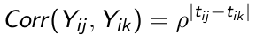](https://bookstack.mitchellhenschel.com/uploads/images/gallery/2023-02/zhLimage.png)
The correlations declines exponentially over time as the distance between pairs of measurements increase, same as in the AR(1) case.
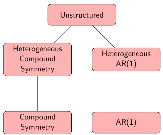
### Choosing a Covariance Pattern Model
When the covariance model A with theta\_a estimated parameters can be written as different covariance structure B (with theta\_b > theta\_a parameters) with certain restrictions imposed, then we say that A is in nested in B.
Ex. the compound symmetry model is nested within an unstructured covariance model. In this case we can test which covariance structure fits the data better by using a likelihood ratio test:
[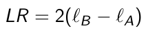](https://bookstack.mitchellhenschel.com/uploads/images/gallery/2023-02/5noimage.png)
where ℓB and ℓA are the maximized REML log-likelihoods. LR follows a chi2theta\_B - theta\_a
[](https://bookstack.mitchellhenschel.com/uploads/images/gallery/2023-02/LXaimage.png)
In many cases, we would like to compare non-nested models. For example, we would like to compare the fit between compound symmetry and AR(1) covariance structures it is not possible to use the LR test but we can use measures of fit for each model:
AIC = -2(ℓ - c)
BIC = -2(ℓ - log(n - p)\*c)
where ℓ is the maximized log-likelihood, c is the number of covariance parameters and n is the number of subjects.