# Marginal Methods
In many biomedical applications outcomes are binary, ordinal or a count. In such cases we consider extension of generalized linear models for analyzing discrete longitudinal data. These non-linear models require that a linear transformation of the mean response can be modeled in a regression setting. The non-linearity raises issues with the interpretation of the regression coefficients.
We let Yi denote the response variable for the ith subject, and:
[](https://bookstack.mitchellhenschel.com/uploads/images/gallery/2023-02/7ayimage.png)
is a p\*1 vector of covariates. A generalized linear model for for Yi needs the following three-part specification:
##### 1. A Distributional Assumption
Generalized linear models assume that the response variable has a probability distribution belonging to the exponential family (normal, bernoulli, binomial or Poisson). A feature of the exponential family is the variance can be expressed as:
[](https://bookstack.mitchellhenschel.com/uploads/images/gallery/2023-02/qjhimage.png)
Where phi is a dispersion parameter and v(μi) is the variance function. For example:
- Variance function of normal distribution: v(μ) = 1
- Variance function of Bernoulli: v(μ) = μ(1 - μ)
##### 2. A Link Function
The link function g(.) applies to the mean and then links the covariates to the transformed mean η such that:
[](https://bookstack.mitchellhenschel.com/uploads/images/gallery/2023-02/jSAimage.png)
For example, the canonical link functions for some common distributions are:
[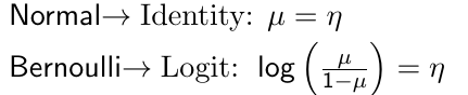](https://bookstack.mitchellhenschel.com/uploads/images/gallery/2023-02/Z5Zimage.png)
##### 3. A Systematic Component
The systematic component specifies the effects of the covariates Xi on the mean of Yi can be expressed in terms of the following linear predictor:
[](https://bookstack.mitchellhenschel.com/uploads/images/gallery/2023-02/piGimage.png)
Note that the term 'linear' refers to the regression parameters.
#### Binary response
Let Yi denote a binary response variable with two categories such as presence or absence of a disease. The probability distribution is Bernoulli with Pr(Yi = 1) = μi and Pr(Yi = 0) = (1 - μi). Using the logit as the link function we have:
[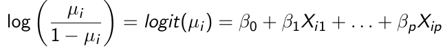](https://bookstack.mitchellhenschel.com/uploads/images/gallery/2023-02/s9jimage.png)
Where μi / (1 - μi) are the odds of success
A unit change of Xik changes the odds of success *multiplicitively* by a factor of exp(βk).
The logistic regression model can be derived from the notion of a latent variable model. Suppose that Li is a latent continuous variable which follows a standard logistic distribution (0, π2/3) and that a positive response is observed only when Li exceeds some threshold τ , such that:
[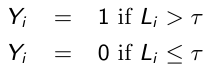](https://bookstack.mitchellhenschel.com/uploads/images/gallery/2023-02/wviimage.png)
It can be shown that:
[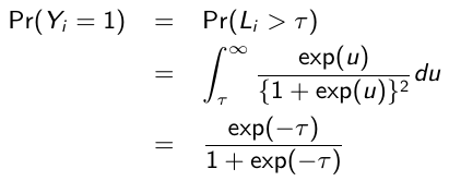](https://bookstack.mitchellhenschel.com/uploads/images/gallery/2023-02/LUtimage.png)
### Marginal Models
Suppose Y'i = (Yi1, Yi2 ..., Yip), a vector of correlated responses from the ith subject. To analyze such correlated data we must specify or make assumptions about the multivariate or joint distribution, and to do so we will consider these main extensions of GLM: Marginal Models and Mixed Effects Models (next lecture)
A marginal model for longitudinal data has the following three-part specification:
1. E(Yij | Xij) = μij is assumed to depend on the covariates through a known link function:
[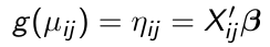](https://bookstack.mitchellhenschel.com/uploads/images/gallery/2023-02/Feqimage.png)
2. We also identify a known variance function:
[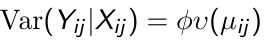](https://bookstack.mitchellhenschel.com/uploads/images/gallery/2023-02/Mx8image.png)
Where phi is a scale parameter that may be constant or may vary at each measurement occasion.
3. The conditional within-subject association among the response measurements, given the covariates, is assumed to be a function of an additional set of association parameters, α.
Note that the systematic component is the key building block of a marginal model and specifies the model for the mean response at each occasion, E(Yij | Xij), and its dependence on the covariates. Marginal responses also assume that the conditional mean of the jth response given Xi1, ..., Xin depends only on Xij:
[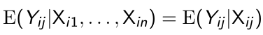](https://bookstack.mitchellhenschel.com/uploads/images/gallery/2023-02/5I5image.png)
With time-invariant or fixed time-varying covariates this assumption holds. It does not hold when a time-varying covariate varies randomly over time.
Note on association: We avoid using the term correlation. This is because 1) correlation is not a natural measure of within-subject association for discrete responses, and 2) the joint distribution of discrete responses is not often well specified or not easily tractable.
### Generalized Estimating Equation
Since there is no convenient or natural specification of the joint multivariate distribution of Yi for marginal models when the responses are discrete, we need an alternative to the Maximum Likelihood estimation. In 1986 Liang and Zeger proposed such a method based on the concept of 'estimating equations' which provides a general and unified approach for analyzing discrete and continuous responses with marginal models. For linear models Generalized Least Sqaures is a special case of estimating equations, for non-linear models the approach is called Generalized Estimating Equations (GEE).
Given a model for the pairwise correlations, the covariance matrix can be expressed as:
[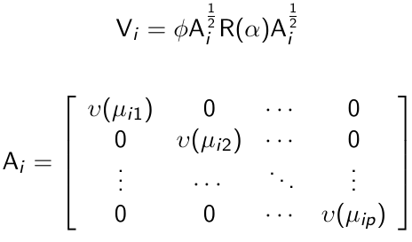](https://bookstack.mitchellhenschel.com/uploads/images/gallery/2023-02/DIMimage.png)
And R(α) is the correlation matrix. Vi is known as a working covariance matrix to distinguish it from the true underlying covariance matrix.
#### Generalized Estimating Equations
An estimate of β can be obtained as the solution of the following generalized estimating equations:
[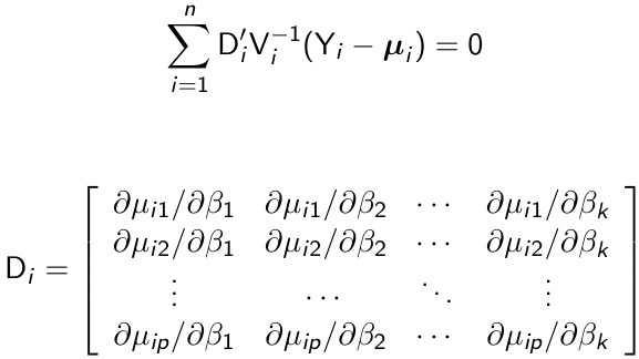](https://bookstack.mitchellhenschel.com/uploads/images/gallery/2023-02/JAEimage.png)
Di can be thought of as a matrix that transforms from the original units of μij to the units of g(μij)
The generalized estimating equations are functions of both β and α and in general have no closed-form solution. In this case, the following two-stage estimation procedure is required:
1. Given current estimates of α and φ, Vi is estimated and an updated estimate of β is obtained as the solution of GEE
2. Given the current estimate of β updated estimates of α and φ are obtained based on the standardized residuals:
[](https://bookstack.mitchellhenschel.com/uploads/images/gallery/2023-02/Xuuimage.png)
For example, φ can be estimated by:
[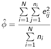](https://bookstack.mitchellhenschel.com/uploads/images/gallery/2023-02/YVIimage.png)
α can be estimated in a similar way:
[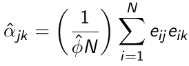](https://bookstack.mitchellhenschel.com/uploads/images/gallery/2023-02/bDlimage.png)
And steps 1 and 2 are repeated until convergence
#### Properties of GEE Estimators
β̂\_hat is a consistent estimate of β̂, with very high probability and sufficiently large N then β̂\_hat ~= β̂. The consistency of β̂\_hat depends on the correct specification off the mean, but it still holds even if the covariance of Yi has been mispecified.
[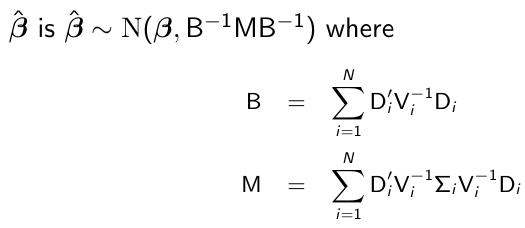](https://bookstack.mitchellhenschel.com/uploads/images/gallery/2023-02/Dsgimage.png)
By replacing Di, Vi, and sigma\_i by their estimates, we get the empirical or sandwich estimator. Note that if we model Vi correctly then Vi = Sigma\_i and Var(β̂) = B-1
#### Daignostics
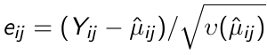
We can easily calculate residuals:
[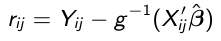](https://bookstack.mitchellhenschel.com/uploads/images/gallery/2023-02/UK2image.png)
Since Var(rij) = f(μij) it is preferable to use studentized residuals:
[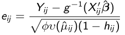](https://bookstack.mitchellhenschel.com/uploads/images/gallery/2023-02/Ot5image.png)
where hij is the leverage of the jth observation on the ith individual and describes the influence each observation has on its own predicted value
We can use diagnostic plots similar to the continuous case to find outlying observations; such as the Mahalonobis-type statistic:
[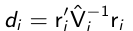](https://bookstack.mitchellhenschel.com/uploads/images/gallery/2023-02/lVsimage.png)
which has a chi-squared distribution if the model for the mean is correctly specified and Vi ~= sigma\_i
## SAS Code
```
* No repeated measures, logistic regression, uses maximum likelihood;
proc logistic data=s857.BPD plots=EFFECT descending;
class BPD;
model BPD=Weight;
title1 'Simple Logistic Regression using PROC LOGISTIC';
run;
* Use GEE, can use if no repeated measures, interpret estimate, never use genmod in non-repeated measures, just here as intro;
proc genmod data=s857.BPD descending;
class BPD;
model BPD=Weight/DIST=binomial LINK=LOGit;
title1 'Simple Logistic Regression using PROC GENMOD';
run;
proc logistic data=s857.BPD plots=EFFECT descending;
class BPD;
model BPD=Weight Gest_Age Toxemia;
title1 'Multiple Logistic Regression using PROC LOGISTIC';
run;
*Repeated measures, y = obesity;
proc genmod data=s857.BPD descending;
class BPD;
model BPD=Weight Gest_Age Toxemia/DIST=BINOMIAL LINK=LOGIT;
title1 'Multiple Logistic Regression using PROC GENMOD';
run;
title1 'Marginal Logistic Regression Model for Obesity';
title2 'Muscatine Coronary Risk Factor Study';
*have increase in prevalence in obesity from 8 to 12 then becoems constant for both genders;
*repeated measures since each person has 4 binary measures (obesity status at 4 ages);
proc freq data=s857.muscatine;
where occasion=2;
by gender;
tables age*y;
run;
*apply quad or cubic model since trend not linear;
* 12 is pop mean, dont want multicollinearity when using quad or cubic in model;
* may use these in the model;
data muscatine;
set s857.muscatine;
cage=age - 12;
cage2=cage*cage;
cage3=cage2*cage;
run;
*quad model with respect to age;
* use repeated statement by id (ppl have mult measurements), that variable should also be in class statement;
*type = compund symmetry, so R(alpha) = [1 p p .. p, p 1 p p, p p 1 p...];
/*using a compound symmetry structure working correlation*/
proc genmod data=muscatine ;
class id occasion;
model y(event='1')=gender cage cage2 / dist=bin link=logit
type3 wald;
repeated subject=id / type=cs corrw covb;
run;
*look at Analysis of GEE Parameter Estimates table, need to exp estimate if want OR;
*corr parameter is 0.54 from output, no clear interpretation;
/*Using Log OR correlation structure*/
*use logor structure, fullclust says go and find all the associations btwn all the different measures (subj have at most 3 diff measurements) 1&3,1&2,2&3;
proc genmod data=muscatine ;
class id occasion;
model y(event='1')=gender cage cage2 / dist=bin link=logit
type3 wald;
repeated subject=id / withinsubject=occasion logor=fullclust;
run;
*look at Analysis of GEE Parameter Estimates table;
*three alphas;
*alpha1 = logOR(Yi1, Yi2), OR(Yi1, Yi2) = P(Yi1 = 1, Yi2 = 1)*P(Yi1 = 0, Yi2 = 0) / (P(Yi1 = 1, Yi2 = 0)*P(Yi1 = 0, Yi2 = 1));
* to find OR exp estimate, is OR of having same outcome in occasion 1 and occasion 2 vs diff outcome;
* alpha2 = logOR(Yi1, Yi2);
* alpha3 = logOR(Yi2, Yi3);
*1,2 and 2,3 are only two years apart;
* maybe want alpha1 = logOR(Yi1, Yi2) = logOR(Yi2, Yi3);
/*Equivalent model*/
* three columns, three alphas;
*first row: for 1 2, this is only alpha1;
*second row: for 1 3, this is only alpha2;
*third row: for 2 3, this is only alpha3;
proc genmod data=muscatine descending;
class id occasion;
model y=gender cage cage2 / dist=bin link=logit
type3 wald;
repeated subject=id / withinsubject=occasion
logor=zrep( (1 2) 1 0 0,
(1 3) 0 1 0,
(2 3) 0 0 1) ;
run;
/*The same association between any two occasions */
* compound symmetry but with logOR presentation;
* only one alpha that is same for (1 2) (1 3) (2 3);
* this parametirazation works if same measurement on same subjects at same time (i.e. age 8, 10, 12 for all) like clinical trial design;
proc genmod data=muscatine descending;
class id occasion;
model y=gender cage cage2 / dist=bin link=logit
type3 wald;
repeated subject=id / withinsubject=occasion
logor=zrep( (1 2) 1 ,
(1 3) 1 ,
(2 3) 1 );
run;
/*Testing whether the association between occasions 1-2
and 2-3 are the same */
* three columns, three alphas;
*first row: for 1 2, this is only alpha1;
*second row: for 1 3, this is only alpha2;
*third row: for 2 3, this is alpha1 + alpha3;
* if alpha3 is zero, then (1 2) is same as (2 3), get rid and only have 2 alphas;
proc genmod data=muscatine descending;
class id occasion;
model y=gender cage cage2 / dist=bin link=logit
type3 wald;
repeated subject=id / withinsubject=occasion
logor=zrep( (1 2) 1 0 0,
(1 3) 0 1 0,
(2 3) 1 0 1) ;
run;
/*Fitting a model with the association between occasions 1-2
and 2-3 are the same */
* store p1 = sotre residuals;
proc genmod data=muscatine descending;
class id occasion;
model y=gender cage cage2 / dist=bin link=logit
type3 wald;
repeated subject=id / withinsubject=occasion
logor=zrep( (1 2) 1 0 ,
(1 3) 0 1,
(2 3) 1 0);
store p1;
run;
* plot predicted values for prevalence for diff genders at diff age for quad model;
ods html style=journal;
proc plm source=p1;
score data = muscatine out=pred /ilink;
run;
proc sort data = pred;
by gender age;
run;
proc sgplot data = pred;
series x = age y = predicted /group=gender;
run;
/*Cubic Model*/
proc genmod data=muscatine descending;
class id occasion;
model y=gender cage cage2 cage3/ dist=bin link=logit
type3 wald;
repeated subject=id / withinsubject=occasion
logor= zrep( (1 2) 1 0,
(1 3) 0 1,
(2 3) 1 0);
store p1;
run;
ods html style=journal;
proc plm source=p1;
score data = muscatine out=pred /ilink;
run;
proc sort data = pred;
by gender age;
run;
proc sgplot data = pred;
series x = age y = predicted /group=gender;
run;
/* Example of a quadratic model with gender age interaction */
proc genmod data=muscatine descending;
class id occasion gender ;
model y=gender cage cage2 gender*cage gender*cage2 / dist=bin link=logit
type3 wald;
contrast 'Age X Gender Interaction' gender*cage 1 -1, gender*cage2 1 -1 /wald;
repeated subject=id / withinsubject=occasion logor=fullclust;
run;
/*********************************
Diagnostics(Optional)
*********************************/
*assess statement = uses bootstrap to look at sum of residuals, should be centered around 0;
proc genmod data=muscatine descending;
class id occasion;
model y=gender cage cage2 cage3/ dist=bin link=logit
type3 wald;
repeated subject=id / withinsubject=occasion
logor=zrep( (1 2) 1 0,
(1 3) 0 1,
(2 3) 1 0);
assess var=(cage)/resamples=10000 seed=7435865;
run;
ods rtf close;
```