# Linear Mixed Effects Models II
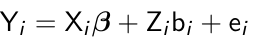
The simplest mixed effect model is a random intercept model where Zi = 1;
[](https://bookstack.mitchellhenschel.com/uploads/images/gallery/2023-02/Kg9image.png)
The random intercept model can be interpreted as the effect of all unobserved subject-specific variables (bi) on the linear predictor.
Random slopes of time-varying covariates (δ) can be interpreted as interaction of unobserved subject specific covariates with observed time-varying covariates.
We can also include a random effect with a time-invariate covariate bi (e.g. treatment group) to produce a heteroscediastic random intercept Zi0 + Zi1bi.
### Two-Stage Formulation
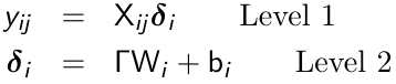
An alternative formulation of the mixed effects models is a two-stage formulation, in which we first specify a within subject or level-1 model where the occasion specific linear predictor is a function of time-varying covariates. Then a between subject or level 2 model is specified:
[](https://bookstack.mitchellhenschel.com/uploads/images/gallery/2023-02/Wj1image.png)
Some elements of δi are constant and some depend only on the observed covariates.
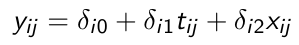
Consider the following with a random intercept and a random slope for time:
[](https://bookstack.mitchellhenschel.com/uploads/images/gallery/2023-02/dzSimage.png)
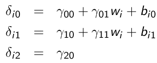
xij is a time-varying covariate and wi is a time-invariant covariate
[](https://bookstack.mitchellhenschel.com/uploads/images/gallery/2023-02/eT7image.png)
The redirected form is obtained by substituting the level-2 model into level-1 model. We then substitute level-2 into level-1 to produce the reduced form with a "cross-level interaction" term γ11witij
- The two formulations are equivalent but it can have an impact on the types of models being considered
- The two-stage formulation encourages inclusion of many cross-level interactions and few same-level interactions
- Due to an abundance of interactions in the two-stage formulation, we usually center around the mean all variables except time. In our example, centering of wi makes γ10 interpretable as the mean effect of tij when tij when wi takes it mean value.
#### Unobserved Confounders
In longitudinal studies, it is often said the "subjects serve as their own controls" when considering time-varying covariates. This seems to imply that all subject-level observed and unobserved covariates have been controlled for, but this is NOT true since this omitted covariates may correlate and hence be confounded with the time-varying variables of interest. If Cov(xij, uij) != 0, then we will have omitted variable bias; We say that xij is *endogenous* or correlated with the random intercept bi0
#### Centering
Cov(xij, uij) = 0 if x\_hat\_i = x\_hat\_j for any i,j; We can then avoid omitted variable bias by subject-mean centering xij, forming the instrumental variable xijd = xij - x\_hat\_i and running the following model:
[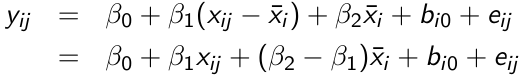](https://bookstack.mitchellhenschel.com/uploads/images/gallery/2023-02/Veuimage.png)
β1 can be interpreted as a purely within-subject (or longitudinal) effect and β2 as between-subject (or cross-sectional) effect. A test of the null hypothesis β1 = β2 is equivalent to the Durbin-Wu-Hausman test for exogeneity.
### Linear Fixed Effects Models
Fixed effects linear models are formulated as:
[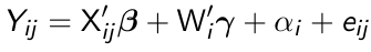](https://bookstack.mitchellhenschel.com/uploads/images/gallery/2023-02/W24image.png)
where X denotes a q\*1 vector of time-varying covariates, Wi denotes a (p-q)\*1 vector of time-invariant covariates and αi are fixed effects representing the time-invariant unobserved confounders, and eij remains the random within-subject errors.
This accounts for all observed/unobserved time-invariate confounders\*, making this a model likely less prone to bias with the obvious drawback of way more terms to estimate (loss of power/degrees of freedom)
\*assuming that the effects on the response remain constant over time
Although this looks very similar to the random intercepts model considered last class, note that in the mixed effects formulation αi are considered *random* while now they are considered *fixed*.
##### Properties of Fixed Effect Models
- Xij is assumed to be strictly exogenous; i.e. current values of the response Yij given Xij do not predict the subsequent value of Xij+1
- The fixed effects αi can be correlated with Xij and Wi unlike mixed effects where αi are assumed independent of Xij and Wi
- Fixed effects models cannot estimate the effects of time-invariant covariates. Since αi and W'iγ are perfectly colinear, the time-invariant covariates are effectively removed from the analysis
- Fixed effects models remove bias when there are unmeasured but stable characteristics of the subjects that are correlated with time-varying covariates of main scientific interest
#### Bias-Variance Trade-Off
Although, under the conditions we discussed the fixed effects model may provide unbiased estimates of the time-varying covariates, they will generally have larger standard errors for those estimated effects than those produced by mixed effects models
Fixed effects base estimation exclusively on the within-subject variation and ignore any between-subject variation, while mixed effects utilize both sources of variability resulting in smaller standard errors.
The greater the proportion of between subject variation in a time-varying covariate, the larger the differences in the magnitudes of the standard errors between mixed and fixed effects models.
#### Comparison of Fixed and Mixed Effects Estimates
Consider the simple random effect model:
[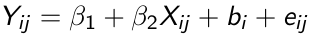](https://bookstack.mitchellhenschel.com/uploads/images/gallery/2023-02/zD0image.png)
It can be shown that the random effects estimator β̂2 RE can be written as:
[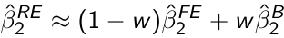](https://bookstack.mitchellhenschel.com/uploads/images/gallery/2023-02/6Bpimage.png)
Where β̂2 FE is the fixed effects estimator and β̂2 B is an estimator based only on between-subject variation and is obtained from the regression of Ȳi on X̄i. w is the weight given by:
[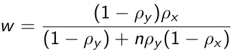](https://bookstack.mitchellhenschel.com/uploads/images/gallery/2023-02/Zjbimage.png)
Where [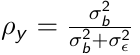](https://bookstack.mitchellhenschel.com/uploads/images/gallery/2023-02/YZNimage.png) is the proportion of variability in the response due to between subject variation and ρx is the corresponding proportion of variability of Xij that is due to between-subject variation.
- When within-subject variation in the response is small then ρy -> 1 which results to w -> 0 and β̂2 RE = β̂2 FE
- When within-subject variation in the covariate is large then ρx -> 1 which results to w -> 0 and β̂2 RE = β̂2 FE
### Residual Analyses and Diagnostics
We define a vector of residuals for each individual as ri = Yi - Xiβ̂
From there a simple scatter plot of the residuals against the predicted mean response or covariates can be observed to see if there are is systemic pattern. The residuals are correlated and usually do not have constant variance.
The standardized residuals are defined as: r\*i =Li-1ri where Li is a lower triangular matrix so that:
[](https://bookstack.mitchellhenschel.com/uploads/images/gallery/2023-02/yw5image.png)
Effectively a Li is a 'square root' \[but for matrices\] of the var/covar matrix.
r*i are uncorrelated and have unit variance*. r\*ik is an estimate of:
[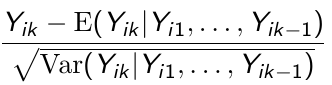](https://bookstack.mitchellhenschel.com/uploads/images/gallery/2023-02/0Xsimage.png)
We can use the standardized residuals to detect outlying observations:
- Scatterplot of standardized residuals against teh predicted means response
- Scatterplot of standardized residuals against covariates
- Normal QQ plot to assess the assumption of normallity
- Compute Mahalanobis distance to detect *outlying individuals:* [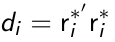](https://bookstack.mitchellhenschel.com/uploads/images/gallery/2023-02/CHjimage.png)
di ~ chi-square distributed with degrees of freedom equal to the number of measurements for individual i
#### Semi-Variogram
We use the semi-variogram to assess the adequacy of a selected model for the covariance.
[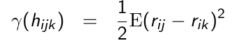](https://bookstack.mitchellhenschel.com/uploads/images/gallery/2023-02/NeDimage.png)
Where hijk = the time elapsed between repeated measurement j and k on the ith individual. Since E(rij) = 0 then:
[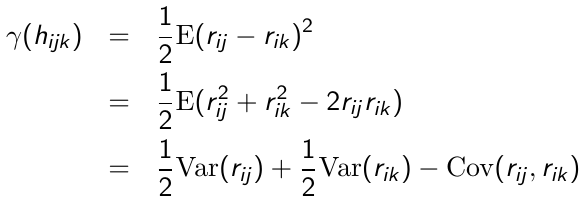](https://bookstack.mitchellhenschel.com/uploads/images/gallery/2023-02/7V0image.png)
So since each r\* has a variance of 1 and covariance of 0, the semi-variogram for r\*ij is:
[](https://bookstack.mitchellhenschel.com/uploads/images/gallery/2023-02/Awlimage.png)
Thus, in a correctly specified model for the covariance the plot of the semi-variogram for the standardized residuals vs. time should fluctuate randomly around a horizontal line centered at 1.
### Model Selection Strategy
We can use the following guidelines for selecting a model for correlated data:
1. Fit a saturated model such as profile analysis
2. For a full model select an appropriate covariance structure using REML. You can use likelihood ratio when appropriate, or AIC/BIC when LRT is not possible
3. For an appropriate covariance structure, select an appropriate set of covariates using ML. As previously seen, use LRT, AIC or BIC
4. For an appropriate set of covariates, select an appropriate covariance structure using REML
5. Repeat steps 3 and 4
Note that REML is used to compare covariance structures to ensure unbiased estimators, ML is used to compare different combinations of covariates because it's more powerful.
## SAS Code
```
/************************************************
* Six cities study of air pollution and health *
*************************************************/
data fev1;
set s857.fev1;
lgfevht=Log_FEV1_-2*logHgt;
run;
*Durbin-Wu-Hausman test;
*Computes mean age by ID, spits it into another dataset;
proc means data=fev1 ;
*where id ne 197;
by id;
var age ;
output out=mean_age;
run;
data mean_age;
set mean_age;
if _STAT_='MEAN' then;else delete;
rename age=age_mean;
keep id age;
run;
data fev1;
merge fev1 mean_age;
by id;
run;
data fev1;
set fev1;
*Creating mean-centered age;
*Prevents confounding with random slope;
age_dev=age-age_mean;
run;
proc means data=fev1 mean var;
var age age_dev;
run;
proc means data=mean_age;
var age_mean;
run;
*RE model;
proc mixed data=fev1 method=ml covtest;
*where id ne 197;
class id;
model lgfevht=age age_mean/s chisq;
random intercept/type=un subject=id G V ;
run;
*Fixed Effects model;
proc glm data=fev1;
*where id ne 197;
class id;
model lgfevht=id age/solution;
run;
quit;
proc mixed data=fev1 method=ml covtest;
*where id ne 197;
class id;
model lgfevht=age /s chisq;
random intercept/type=un subject=id G V;
run;
*To compute rho of Y (the proportion due to within-subject variation in the repsonse;
*Sigma2(b) is UN(1, 1) = 0.01144, Sigma2(e) is Residual = 0.01391;
proc mixed data=fev1 method=ml covtest;
*where id ne 197;
class id;
model lgfevht=/s chisq;
random intercept/type=un subject=id G V ;
run;
proc mixed data=fev1 method=ml covtest;
*where id ne 197;
class id;
model age=/s chisq;
random intercept/type=un subject=id G V ;
run;
/************************************************
Study of influence of menarche on changes in body fat
*************************************************/
proc sgplot data=s857.fat noautolegend ;
* spaghetti plot;
yaxis min = 0 max = 50;
reg x=time_men y=Perc_BF
/ group = id nomarkers LINEATTRS = (COLOR= gray PATTERN = 1 THICKNESS = 1) ;
* overall spline;
reg x=time_men y=Perc_BF
/ nomarkers LINEATTRS = (COLOR= red PATTERN = 1 THICKNESS = 3) ;
run;
quit;
ods graphics on;
proc loess data=s857.fat plots=all;
model Perc_BF = time_men;
run;
ods graphics off;
data fat;
set s857.fat;
knot=max(time_men,0);
run;
ods graphics;
proc mixed data=fat covtest plots=all;
model Perc_BF = time_men knot/s chisq outpred=yhat outpm = pred1f residual;
random intercept time_men knot/type=un subject=id G V ;
run;
/*****************************************
* Mahalanobis Distance *
*******************************************/
data pred1f;
set pred1f;
sqStudentResid=StudentResid**2;
visits=1;
run;
proc means data=pred1f noprint;
*sum command gives sums in order given (sum of sqStudentResid is output as distance, visits as novisits);
var sqStudentResid visits;
output out=mahalanobis (drop=_type_ _freq_)
sum(sqStudentResid visits)=distance novisits;
by id;
run;
data mahalanobis;
set mahalanobis;
pvalue=1-probchi(distance,novisits);
run;
proc print data=mahalanobis;
*Bonferroni correction to p value based on number of tests;
where pvalue<0.05/162;
run;
/*****************************************/
proc means data=fat;
var time_men;
run;
proc variogram data=pred1f outv=outv noprint;
*Computing measurement differences within subjects with measurement differences (i.e., when they were taken) of up to 10 with iterative values of 1;
*first plot (fit plot) shows average within-subject residuals for different lags. Should be randomly distributed around 0, but def shouldn't have a pattern;
compute lagd=1 maxlag=10;
coord xc=time_men yc=visits;
by id;
var StudentResid;
run;
ods graphics on;
proc loess data=outv plots=all;
model variog = distance;
run;
ods graphics off;
/*ALternative model*/
data fat;
set fat;
t=time_men;
run;
*Outpred gives FE (population-level) predictions, and outpm gives subject-level predictions;
proc mixed data=fat covtest plots=all;
class t;
model Perc_BF = time_men knot/s chisq outpred=yhat2 outpm = pred2f residual;
random intercept time_men knot/type=un subject=id G V;
*The added repeated statement assumes the error terms don't have constant variances and is looking for that structure;
repeated t/type=sp(exp)(t) subject=id;
run;
data pred2f;
set pred2f;
sqStudentResid=StudentResid**2;
visits=1;
run;
proc variogram data=pred2f outv=outv2 noprint;
compute lagd=1 maxlag=10;
coord xc=time_men yc=visits;
by id;
var StudentResid;
run;
ods graphics on;
proc loess data=outv2 plots=all;
model variog = distance;
run;
ods graphics off;
```