Introduction to Longitudinal and Clustered Data

Correlated data occurs in a variety of situations. The four basic types:

1. Repeated measurements data
2. Clustered data designs
3. Spatially correlated data
4. Multivariate data

Repeated Measurements

Longitudinal data is a response variable collected from the same individuals over a period of time. Special cases may include cross-over designs and parallel group repeated measures design; For example, a two-period, two treatment design design where each individual received each treatment on 2 different occasions. Correlation obtained from the same person or cluster are usually positively correlated.

• Repeated observations of the response variable on individuals over multiple occasions or under different experimental conditionals allow direct study of the change of the outcome
• The most common case of repeated measurements are longitudinal data
• Longitudinal data requires special statistical techniques because repeated observations are correlated

Clustered Data

Clustered data occurs when observations are grouped in clustered based on a common factor (location, ancestry, clinical factor, etc).

Examples of clustered data include:

• Paired data:
  • Ex. studies on twins where each pair serves as a natural cluster
• Familial studies:
  • Ex. Study of cancer with families as clusters
• Randomized clustered clinical trials:
  • In a rural area with an endemic disease, randomize whether the whole village will receive intervention, rather than individuals

Spatially Correlated Data

Spatially correlated data occurs when observations are associated with a specific location. The proximity of locations determines the extent that the observations are correlated.

Examples of spatially correlated data:

• Epidemiological studies
  • Studies aimed at describing the incidence and prevalence of a particular disease use spacial correlation models in an attempt to smooth out region-specific counts so as to better asses potential environmental determinants and patterns associated with the disease
• Image analysis
  • Image segmentation studies where the goal is to extract information about a particular region of interest from a given image

Multivariate Data

Multivariate data occurs when two or more response variables are measured per experimental unit or individual. There are several methods that deal with multivariate data, such as discriminant analysis, principal component analysis, or factor analysis.

• Multivariate repeated measurements
  • Any study where we have two or more outcome variables measured repeatedly over time
• Joint modeling of repeated measurements and event-times data
  • Studies where draw joint inferences on patient outcomes and any serial trends in a potential biomarker

Explanatory Variable

In correlated data the set of explanatory variables or covariates used to model the mean response can be broadly classified in two categories:

• Within-unit covariates (time-dependent covariates)
  • Sometime that changes over time as the outcomes changes
• Between-unit covariate (time-independent covariate)

Dependence and Correlation

Two random variables  X and Y with marginal density function f_x(X) and f_y(Y) are said to be independent if and only if their joint density function can be written as the produce of the two marginals:
    f_x,y(X,Y) = f_x(X)*f_y(Y)

Alternatively X and Y are independent if the conditional distribution of Y given X does not depend on X:
    f_y(Y|X) = f_y(Y)

Two variables are uncorrelated if:
    E[(Y - μY)(X - μX)] = 0

E[(Y - μY)(X - μX)] is called the covariance, which can take any positive or negative value depending on the units. To make it unit independent and get the correlation we divide it by the standard deviations of the two variables:

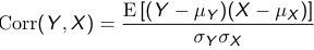
Correlation must be between -1 and 1

Note that independent variables are uncorrelated but variables can be uncorrelated without being independent.

Covariance Matrix

Let Y_ij be the j^th measurement of the i^th subject. We collect all observations in a vector (Y_i1, Y_i2, ... Y_ip) we define the covariance matrix as the following array of variances and covariances: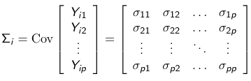

For example, Cov(Y_i1, Y_i2) = 𝜎₁₂ is the covariance between the first and second repeated measure of the i^th subject.

SAS Code

libname S857 'C:\Users\yorghos\Dropbox\Courses\BS857\2021\Datasets';
data lead;
set s857.tlc;
y=y0;time=0;output;
y=y1;time=1;output;
y=y4;time=4;output;
y=y6;time=6;output;
drop y0 y1 y4 y6;
run;

ODS graphics on;
Proc Glimmix data=lead;
class time TRT;
model y =time TRT time*trt;
lsmeans time*trt
/ plots=(meanplot( join sliceby=trt)); 
run;
ODS graphics off;
ods rtf close;

proc corr data=s857.tlc cov;
var y0 y1 y4 y6;
run;

/*Repeated Measures MANOVA*/
proc mixed data=lead;
class id trt time;
model y=trt time trt*time/s chisq;
repeated time/type=un subject=id r rcorr;
run;


proc mixed data=lead method=ML;
class id trt (ref='P') time(ref="0");
model y=trt time trt*time/s  ;
repeated time/type=un subject=id r rcorr ;
estimate 'TRT a time 0' int 1 trt 1 0 time 0 0 0 1 trt*time  0 0 0 1 0 0 0 0;
estimate 'TRT a time 6' int 1 trt 1 0 time 0 0 1 0 trt*time 0 0 1 0 0 0 0 0 ;
estimate 'TRT a time 4' int 1 trt 1 0 time 0 1 0 0 trt*time 0 1 0 0  0 0 0 0;
estimate 'TRT a time 1' int 1 trt 1 0 time 1 0 0 0 trt*time  1 0 0 0 0 0 0 0;

estimate 'TRT Change Time 1 - Time 0' time 1 0 0 -1 trt*time  1 0 0 -1 0 0 0 0;

run;