Analysis of Correlated Data
BS857: Modern methods for analyzing correlated observations in a regression framework. This course covers the design, analysis, and interpretation of correlated data studies with an emphasis on longitudinal studies. Unfortunately, my professor had no teaching ability so these notes come from publicly available resources.
- Introduction to Longitudinal and Clustered Data
- Response Profile Analysis
- Modeling the Mean and Covariance
- Linear Mixed Effects Models I
- Linear Mixed Effects Models II
- Marginal Methods
- Generalized Linear Mixed Effects Models
- Multi-Level Modeling
- Multiple Imputation
- Mutlivariate and Joint Models for Longitudinal Data
- Time Series Models
Introduction to Longitudinal and Clustered Data
Correlated data occurs in a variety of situations. The four basic types:
- Repeated measurements data
- Clustered data designs
- Spatially correlated data
- Multivariate data
Repeated Measurements
Longitudinal data is a response variable collected from the same individuals over a period of time. Special cases may include cross-over designs and parallel group repeated measures design; For example, a two-period, two treatment design design where each individual received each treatment on 2 different occasions. Correlation obtained from the same person or cluster are usually positively correlated.
- Repeated observations of the response variable on individuals over multiple occasions or under different experimental conditionals allow direct study of the change of the outcome
- The most common case of repeated measurements are longitudinal data
- Longitudinal data requires special statistical techniques because repeated observations are correlated
Clustered Data
Clustered data occurs when observations are grouped in clustered based on a common factor (location, ancestry, clinical factor, etc).
Examples of clustered data include:
- Paired data:
- Ex. studies on twins where each pair serves as a natural cluster
- Familial studies:
- Ex. Study of cancer with families as clusters
- Randomized clustered clinical trials:
- In a rural area with an endemic disease, randomize whether the whole village will receive intervention, rather than individuals
Spatially Correlated Data
Examples of spatially correlated data:
- Epidemiological studies
- Studies aimed at describing the incidence and prevalence of a particular disease use spacial correlation models in an attempt to smooth out region-specific counts so as to better asses potential environmental determinants and patterns associated with the disease
- Image analysis
- Image segmentation studies where the goal is to extract information about a particular region of interest from a given image
Multivariate Data
Multivariate data occurs when two or more response variables are measured per experimental unit or individual. There are several methods that deal with multivariate data, such as discriminant analysis, principal component analysis, or factor analysis.
- Multivariate repeated measurements
- Any study where we have two or more outcome variables measured repeatedly over time
- Joint modeling of repeated measurements and event-times data
- Studies where draw joint inferences on patient outcomes and any serial trends in a potential biomarker
Explanatory Variable
- Within-unit covariates (time-dependent covariates)
- Sometime that changes over time as the outcomes changes
- Between-unit covariate (time-independent covariate)
Dependence and Correlation
Two random variables X and Y with marginal density function fx(X) and fy(Y) are said to be independent if and only if their joint density function can be written as the produce of the two marginals:
fx,y(X,Y) = fx(X)*fy(Y)
Alternatively X and Y are independent if the conditional distribution of Y given X does not depend on X:
fy(Y|X) = fy(Y)
Two variables are uncorrelated if:
E[(Y - μY)(X - μX)] = 0
E[(Y - μY)(X - μX)] is called the covariance, which can take any positive or negative value depending on the units. To make it unit independent and get the correlation we divide it by the standard deviations of the two variables:
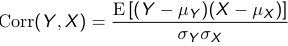
Correlation must be between -1 and 1
Note that independent variables are uncorrelated but variables can be uncorrelated without being independent.
Covariance Matrix
Let Yij be the jth measurement of the ith subject. We collect all observations in a vector (Yi1, Yi2, ... Yip) we define the covariance matrix as the following array of variances and covariances: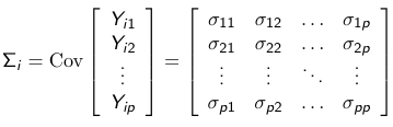
For example, Cov(Yi1, Yi2) = 𝜎12 is the covariance between the first and second repeated measure of the ith subject.
SAS Code
libname S857 'C:\Users\yorghos\Dropbox\Courses\BS857\2021\Datasets';
data lead;
set s857.tlc;
y=y0;time=0;output;
y=y1;time=1;output;
y=y4;time=4;output;
y=y6;time=6;output;
drop y0 y1 y4 y6;
run;

ODS graphics on;
Proc Glimmix data=lead;
class time TRT;
model y =time TRT time*trt;
lsmeans time*trt
/ plots=(meanplot( join sliceby=trt));
run;
ODS graphics off;
ods rtf close;

proc corr data=s857.tlc cov;
var y0 y1 y4 y6;
run;

/*Repeated Measures MANOVA*/
proc mixed data=lead;
class id trt time;
model y=trt time trt*time/s chisq;
repeated time/type=un subject=id r rcorr;
run;


proc mixed data=lead method=ML;
class id trt (ref='P') time(ref="0");
model y=trt time trt*time/s  ;
repeated time/type=un subject=id r rcorr ;
estimate 'TRT a time 0' int 1 trt 1 0 time 0 0 0 1 trt*time  0 0 0 1 0 0 0 0;
estimate 'TRT a time 6' int 1 trt 1 0 time 0 0 1 0 trt*time 0 0 1 0 0 0 0 0 ;
estimate 'TRT a time 4' int 1 trt 1 0 time 0 1 0 0 trt*time 0 1 0 0  0 0 0 0;
estimate 'TRT a time 1' int 1 trt 1 0 time 1 0 0 0 trt*time  1 0 0 0 0 0 0 0;

estimate 'TRT Change Time 1 - Time 0' time 1 0 0 -1 trt*time  1 0 0 -1 0 0 0 0;

run;
Response Profile Analysis
- Are the mean response profiles similar in the groups, or in other words, are the mean response profiles parallel?
This is a question that concerns the group × time interaction effect - Assuming that the mean response profiles are parallel, are the means constant over time?
This is a question that concerns the time effect. - Assuming that the mean response profiles are parallel, are they at the same level?
This is a question that concerns the group effect.
Generalized Least Squares (GLS)
GLS is an extension of ordinary least squares (OLS) since it seeks to minimize a weighted sum of squared residuals. Unlike OLS, GLS accommodates heterogeneity and correlation via the weights which correspond to the inverse of the variance-covariance matrix. The parameters are estimated by minimizing the GLS objective function: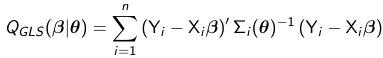
Theta is a vector of variance-covariance parameters. and 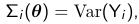
We distinguish 2 cases, where theta is known and theta is not known.
Theta is Known
From calculus we know that in order to minimize the objective function we
1. Differentiate with respect to beta
2. Set the result to 0
3. Solve for beta
The solution to the minimization of the problem is: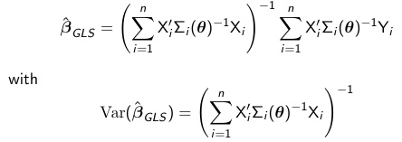
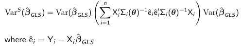
Since assuming we know the variance-covariance matrix of Y is a rather strong assumption we should protect ourselves against model mis-specification. We can use for inference the empirical "sandwich" estimator which is robust:
Theta is Unknown
When theta is unknown we need to replace it in the GLS formulas with a consistent estimate theta_hat. Typically theta_hat = theta_hat*beta_hat_0, where beta_hat_0 is an initial unbiased estimate of beta, such as the OLS estimate and theta_hat*beta_hat_0 is a non-iterative method of moments (MM) type estimator that is consistent for theta. Then the estimated generalized least squares estimator (ELGS) is: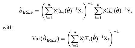
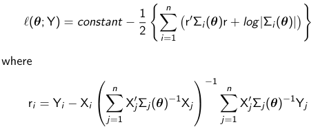
Maximum Likelihood
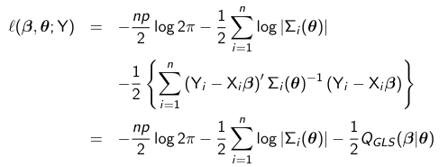
The most common approach to estimation is the method of maximum likelihood. The idea is to use an estimate of beta with the values that are most likely. Given that Y is assumed to have a conditional distribution that is multivariate normal we must maximize the following log-likelihood function:
Maximum Likelihood Estimators (MLE)
When theta is known and fixed the ML and GLS estimators are equivalent. When theta is unknown ML and EGLS estimators are equivalent if theta_hat (in EGLS) is equal to the ML estimate of theta. The MLE is estimated iteratively (as opposed to non-iteratively by EGLS) by maximizing the profile log-likelihood:
Variance of MLE
The variance of the MLE estimate beta_hat_MLE is: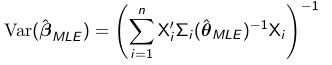
Similarly to GLS we can have a more robust "sandwich" estimator that can be used for inference:
Restricted Maximum Likelihood (REML)
In small samples, ML estimation generally leads to small sample bias in the estimated variance components. To account for the fact that we have uncertainty from estimating beta, we can get unbiased estimates for the variance by maximizing the restricted profile log likelihood:
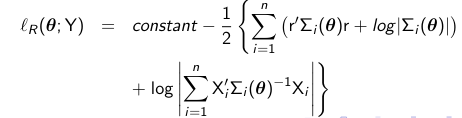
Variance of REML
Similar to other estimation procedures the variance of the REML estimate of beta_hat_REML is: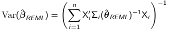
We also have a robust "sandwich" estimator that can be used for inference:
Inference
Consider the following linear representation of a response profile model: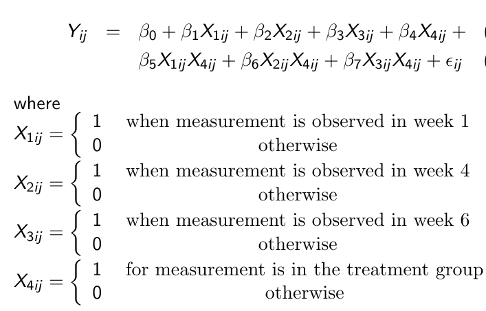
This gives us the following hypotheses:
- Group x Time Interaction Effect
Ex. H0: Beta_5, Beta_6, Beta 7 = 0 vs H1: At least one does not equal 0 - Time Effect
Ex. H0: Beta_1 = Beta_2 = Beta_3 vs H1: Beta_1, Beta_2, Beta_3 are not equal - Group Effect
Ex. H0: Beta_4 = 0 vs H1: Beta_4 != 0
A large sample test for the general linear hypothesis:
H0: L*Beta = 0; H1: L*Beta != 0
can be carried out using the Wald chi-square test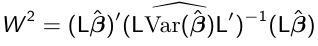
Where L is a r x p matrix of r contrasts or rank r <= p. If we want to test H0: Beta_5, Beta_6, Beta 7 = 0 for group*interaction effect: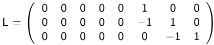
It can be shown that W2 -> chi-squared(r) as n approaches infinity.
Another more robust approach is to replace var(beta_hat) with the robust sandwich estimator, varr(beta_hat). However, there may be a loss in efficiency compared to the model-based estimator.
Contrasts from Baseline
In clinical trials, baseline response is independent from treatment, which means the groups have the same mean response at baseline. In this setting, we may be more interested in testing for equality of the difference between the average responses post-baseline and the baseline value in the two groups.
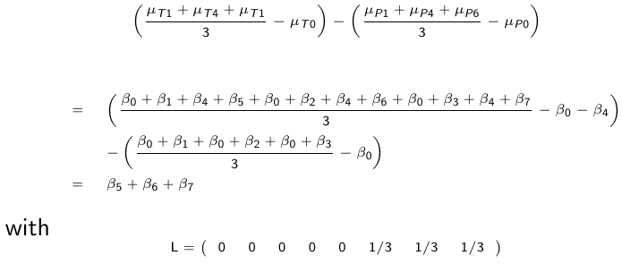
We can test it using the Wald test, which is W2 -> chi2(1)
Area Under the Curve
Instead of comparing the difference of the average post-baseline responses, we can compare the area under the curve minus baseline (AUC). This corresponds to a calculation of the area under the trapezoidal curve.
Baseline as Covariate
An efficient way for testing group differences in a longitudinal clincal trial is to remove the baseline measure from the response and use it as a covariate in the post-baseline responses instead:
Strengths and Weaknesses
+ Is conceptually straightforward
+ It allows arbitrary patterns in the mean response over time
+ It allows for missing values in the response
+ There are various ways to adjust for the baseline
- Repeated measures must be obtained at the same sequence of time for all participants
- It ignores the time ordering of the repeated measures in a longitudinal study
- It may have low power to detect group differences in specific patterns of the mean response over time
- The number of estimated parameters grows rapidly with the number of measurement occasions
Modeling the Mean and Covariance
Suppose we have a model of mean response as a product of time on a continuous value:
The top is control and bottom is treatment. By allowing an index for the jth measurement we allow participants to have measurement in unequal time periods.
Consider the 3 hypotheses which could be tested:
- H0: β3 = 0 for testing parallelism between groups
- H0: β1 = 0 for testing flatness of change over time
- H0: β2 = 0 for testing differences between groups
Quadratic Trends
Higher order terms should be tested (and removed from the model if appropriate) before the lower order terms
In the above we would first test β2 = 0 and if this fails to be rejected we can remove the term and test β1 = 0
To avoid potential problems with collinearity we center the variable of time around their mean before squaring it in order to include it as a quadratic term
Linear Splines
There are application in which the mean response cannot be modeled accurately using a polynomial, like when the mean response increases rapidly for some duration and then more slowly thereafter. In such a case a linear spline model would be appropriate.
Assume the mean response follows a linear trend, but the parameters change at a known time point t*; We can write the following linear spline model with a knot at time t*
We can then write the model separately for each group before and after t*
We can test the following hypotheses:
- H0: β3 = β5 = 0 for testing differences in patterns of change
- H0: β3 = 0 for testing group differences in patterns of change prior to t*
- H0: β4 = β5 = 0 for testing changes in the linear trend model after t*
Comparing Nested Models
When comparing nested models with respect to mean response, we can compute a likeliood ratio test (LTR) by running an ML (not REML) under the two models; full and reduced.
For example:
testing for β2 = 0 is given by:
LTR = 2 (ℓ(β1, β2) - ℓ(β2))
For non-nested models we can use AIC or BIC:
AIC = -2(ℓ - c)
BIC = -2(ℓ - log(n)*c)
Where ℓ is the maximized log-likelihood, c is the number of regression parameters and n is the number of subjects. Select the model that minimized AIC or BIC. The disadvantage of this method is they are empirically/evidence based and we cannot use them to perform any inference.
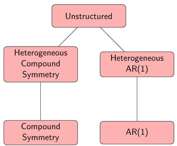
Covariance Pattern Models
One of the most important aspects in modeling correlated data is estimating the covariance structure between measurement occasions. There is no single way of modeling the covariance structure, and a balance needs to be found when imposing structure.
- Too little structure may lead to many parameters for limited data, adversely effecting precision of β
- Too much structure improves β precision but increases the risk of mis-specification that could result in misleading inferences
Unstructured Covariance
For p measurement occasions:
The covariance matrix must always be symmetric and positive-definite. The latter condition ensures that even though the repeated measurements can be highly correlated, none of them can be expressed as a linear combination of the others.
+ No explicit structure required for the covariance among the repeated measures
+ Can handle non-constant variance
- Unstructured covariance has (p*(p+1))/2 parameters. Even for a moderate number of repeated measurements the number of parameters needed to be estimated could be large
- Requires all individuals have the same measurement occasions. No irregular intervals
Compound Symmetry
For p measurement occasions, the compound symmetry model has the following form: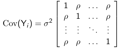
+ Very parsimonious, with only two parameters to be estimated regardless of the measurement occasions
+ Very appealing for certain designs, such as cluster sampling
- Requires strong assumption that the correlation between any pair of measurements to be the same no matter how large the time interval between the measurement is
- Assumes constant variance over time
Heterogeneous Compound Symmetry
For p measurement occasions, the heterogeneous compound symmetry model has the following form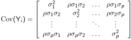
This is a more flexible structure than CS, since it allows non-constant variance but with a smaller number of parameters to be estimated compared to unstructured covariance
First-Order Autoregressive Structure
For p measurement occasions the unstructured covariance has the following form: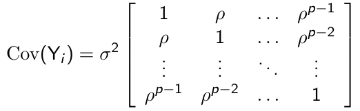
+ Very parsimonious, with only two parameters to be estimated regardless of the measurement occasions
+ Appealing for longitudinal studies since the correlations decline over time as the distance between pairs of measurements increases
- Requires all measurements to be made at equal intervals of time
- Assumes constant variance over time
Heterogenous First-Order Autoregressive Structure
The constant variance assumption can be relaxed and we can have a heterogeneous AR(1) covariance pattern model: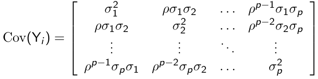
Exponential Structure
When measurements are not equally spaced over time the AR(1) covariance structure can be reformulated as an exponential structure. Let {ti1 ... tip} denote the observation time for subject i, and assume variance is constant across measurement occasions
The correlations declines exponentially over time as the distance between pairs of measurements increase, same as in the AR(1) case.
Choosing a Covariance Pattern Model
When the covariance model A with theta_a estimated parameters can be written as different covariance structure B (with theta_b > theta_a parameters) with certain restrictions imposed, then we say that A is in nested in B.
Ex. the compound symmetry model is nested within an unstructured covariance model. In this case we can test which covariance structure fits the data better by using a likelihood ratio test: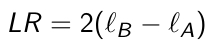
where ℓB and ℓA are the maximized REML log-likelihoods. LR follows a chi2theta_B - theta_a
In many cases, we would like to compare non-nested models. For example, we would like to compare the fit between compound symmetry and AR(1) covariance structures it is not possible to use the LR test but we can use measures of fit for each model:
AIC = -2(ℓ - c)
BIC = -2(ℓ - log(n - p)*c)
where ℓ is the maximized log-likelihood, c is the number of covariance parameters and n is the number of subjects.
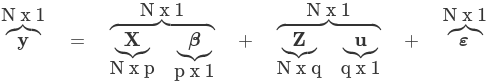
Linear Mixed Effects Models I
Here we'll be considering an alternative approach for analyzing longitudinal data using linear mixed effects models. These models have some subset of the individual parameters vary randomly from one subject to another, thereby accounting for sources of natural heterogeneity in the population.
- Fixed effects are the population characteristics that are assumed to be shared by all subjects
- Random effects are characteristics, unique for each subject
- The combination of both gives rise to mixed effect models
We can write the linear mixed effects model as:
Yi = Xi β + Zibi + ei
Where:
- β is a s*1 vector of fixed effects
- bi is a q*1 vector of random effects (which follows ~N(0, G) we will see below)
- ei is an ni*1 vector of within subject errors (~N(0, Ri)),
- Xi is an ni*s matrix of covariates,
- Zi is a ni*q matrix of covariates with q <= s
We usually assume Ri = σ2In, where In is an ni*ni identity matrix with bi and ei mutually independent.
Model Formulation
The simplest mixed effects model for longitudinal data is:![]()
Where bi (some random intercept) and eij (error) are independent.
The marginal mean response in the population is: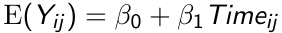
The response for the ith subject at the jth measurement occasion differs from the population mean response by a subject effect bi, and a within subject measurement error eij.
The conditional mean response for any individual:![]()
The residuals of profile analysis and parametric curves (ϵij) and parametric curves such that ϵij = bi + eij
Variance and Covariance Structure
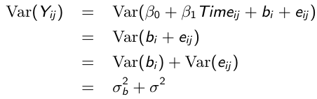
Similarly, the marginal covariance between any pair of responses: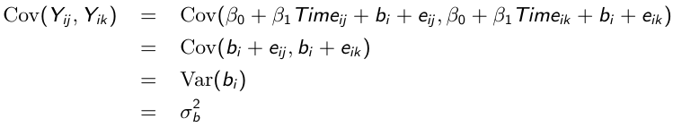
With some linear algebra we can write the variance-covariance matrix as follows: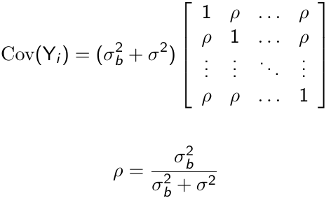
Where ρ is called the intra-cluster correlation coefficient. For ρ > 0, the random intercept mixed effects model is observationally equivalent to a compound symmetry model.
Random Intercept and Slope Model
As the name suggests, this adds a random effect for both the slope and intercept.
Consider the following model:![]()
Where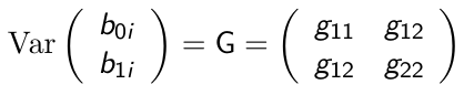
So the variance of each response varies with the time it was taken: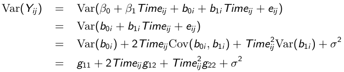
And likewise the covariance between any pair of responses: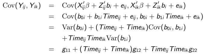
Comparing Mixed Effects Models
Inference with respect to random and fixed effects can be carried out using methods described in the previous lecture for the marginal models. For the nested models, a LR test with REML may be used (which follows a chi-squared dist with 2 degrees of freedom) while non-nested models use AIC or BIC.
Empirical BLUP
In some cases we are interested in subject-specific rather than population-averaged predictions. Mixed effect models are appropriate for this analysis. The empirical best linear unbiased predictor (BLUP) of bi conditional on the observed vector of responses Yi is given by:![]()
![]()
Given the empirical BLUP, b^i the ith subject's predicted mean is: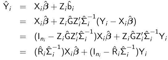
- The empirical BLUP is a weighted average of the population-averaged mean Xibeta_hat and the observed response of the ith subject, Yi
- The empirical BLUP shrinks the ith subject's predicted mean towards the population-averaged mean
- The amount of shrinkage depends on teh relative magntude of the within-subject variability Ri relative to the sum from i, varying weight is assigned to the population-averaged mean Xibeta_hat
Conclusion
- Unlike the models we have seen up to now, mixed effects models explicitly distinguish between-subject and within-subject sources of variability.
- The induced covariance structure is very parsimonious, with only a few number of parameters
- They can be used to predict subject-specific mean response trajectories over time
- They are very flexible in accommodating any kind of imbalance in the data, including the number and timing of measurement occasions.
SAS Code
/************************************************
* Six cities study of air pollution and health	*
*************************************************/
data fev1;
set s857.fev1;
lgfevht=Log_FEV1_-logHgt;
t=age;
run;
proc sgplot data=fev1  noautolegend ;
	* spaghetti plot;
	yaxis min = -0.3 max = 1;
	reg x=age y=lgfevht
    / group = id nomarkers LINEATTRS = (COLOR= gray PATTERN = 1 THICKNESS = 1) ;
	* overall spline;
	reg x=age y=lgfevht
    / nomarkers LINEATTRS = (COLOR= red PATTERN = 1 THICKNESS = 3) ;
run;
quit;
proc mixed data=fev1 covtest;
class t;
model Log_FEV1_=age logHgt Init_Age logInitHgt/s chisq;
repeated  t/type=cs subject=id R Rcorr;
run;
proc mixed data=fev1 covtest method=REML;
model Log_FEV1_=age logHgt Init_Age logInitHgt/s chisq ;
random intercept /type=un subject=id G V;
run;
proc mixed data=fev1 covtest method=REML;
model Log_FEV1_=age logHgt Init_Age logInitHgt/s chisq;
random intercept age/type=un subject=id G V;
run;

proc mixed data=fev1 covtest;
model Log_FEV1_=age logHgt Init_Age logInitHgt/s chisq;
random intercept logHgt/type=un subject=id G V;
run;


proc mixed data=fev1 covtest method=REML;
model Log_FEV1_=age logHgt Init_Age logInitHgt/s chisq;
random  intercept age logHgt/type=un subject=id G V;
run;

/************************************************
* Study of influence of menarche on changes in body fat *
*************************************************/

proc sgplot data=s857.fat  noautolegend ;
	* spaghetti plot;
	yaxis min = 0 max = 50;
	reg x=time_men y=Perc_BF
    / group = id nomarkers LINEATTRS = (COLOR= gray PATTERN = 1 THICKNESS = 1) ;
	* overall spline;
	reg x=time_men y=Perc_BF
    / nomarkers LINEATTRS = (COLOR= red PATTERN = 1 THICKNESS = 3) ;
run;
quit;

   ods graphics on;

   proc loess data=s857.fat plots=all;
      model Perc_BF = time_men;
   run;
 ods graphics off;

 data fat;
 set s857.fat;
 knot=max(time_men,0);
 run;
ods output solutionr=bluptable;
*ods trace on;
*ods listing;
 proc mixed data=fat covtest;
 model Perc_BF = time_men knot/s chisq outpred=yhat outpm = pred1f;
 random intercept time_men knot/type=un subject=id G V solution;
run;
*ods trace off;
ods close;

data yhat;
set yhat;
rename Pred=Pred_r;
run;
data Prediction;
merge yhat pred1f;
keep id pred pred_r time_men perc_BF;
run;

data prediction_long;
length Scale $20;
set prediction;
y=pred;Scale="Average prediction";output;
y=pred_r;Scale="Subject prediction";output;
y=perc_bf;Scale="Raw Data";output;
run;
goptions reset=all;
symbol1 c=blue  v=star   h=.8 i=j      w=5;
symbol2 c=red   v=dot    h=.8 i=j      w=1;
symbol3 c=green   v=squarefilled    h=.8 i=j      w=1;
axis1 order=(0 to 50 by 10) label=( 'Predicted % Body Fat');

proc gplot data=Prediction_long;
where id=10;
plot y*time_men=Scale/ vaxis=axis1 ;
run;
quit;

/************************************************
* Repeated CD4 counts data from AIDS clinical trial.*
*************************************************/
data CD4;
set s857.CD4;
knot=max(week-16,0);
if trt=. then treatment=.;
else if trt<4 then treatment=1;
else treatment=2;
run;
 ods graphics on;

proc transreg ss2 data=cd4;
      model identity(log_cd4) = class(treatment / zero=none) *
                          smooth(week / sm=80);
      output p;
   run;

 ods graphics off;
proc mixed data=cd4 covtest;
class treatment;
model log_cd4=week knot treatment*week treatment*knot/s chisq;
random intercept  week knot/type=un subject=id G V;
run;

proc mixed data=cd4 covtest;
class treatment;
model log_cd4= week knot treatment*week treatment*knot/s chisq;
random intercept  week knot/type=un subject=id G V;
contrast'Interaction test' treatment*week 1 -1,
							treatment*knot 1 -1;
contrast 'Slope test' treatment*week 1 -1  treatment*knot 1 -1;
run;

proc mixed data=cd4 covtest;
class treatment;
model log_cd4=week knot treatment*week treatment*knot Age Gender/s chisq outpred=random;
random intercept  week knot/type=un subject=id G V solution;
ods output solutionr=sr(keep=effect subject estimate probt);
run;
proc print data=sr;
where effect='Week' and Estimate<0 and probt<0.05;
run;
Linear Mixed Effects Models II
The simplest mixed effect model is a random intercept model where Zi = 1; 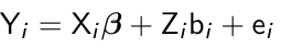
The random intercept model can be interpreted as the effect of all unobserved subject-specific variables (bi) on the linear predictor.
Random slopes of time-varying covariates (δ) can be interpreted as interaction of unobserved subject specific covariates with observed time-varying covariates.
We can also include a random effect with a time-invariate covariate bi (e.g. treatment group) to produce a heteroscediastic random intercept Zi0 + Zi1bi.
Two-Stage Formulation
An alternative formulation of the mixed effects models is a two-stage formulation, in which we first specify a within subject or level-1 model where the occasion specific linear predictor is a function of time-varying covariates. Then a between subject or level 2 model is specified: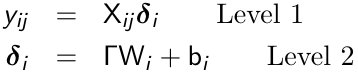
Some elements of δi are constant and some depend only on the observed covariates.
Consider the following with a random intercept and a random slope for time: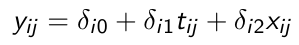
xij is a time-varying covariate and wi is a time-invariant covariate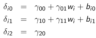
The redirected form is obtained by substituting the level-2 model into level-1 model. We then substitute level-2 into level-1 to produce the reduced form with a "cross-level interaction" term γ11witij
- The two formulations are equivalent but it can have an impact on the types of models being considered
- The two-stage formulation encourages inclusion of many cross-level interactions and few same-level interactions
- Due to an abundance of interactions in the two-stage formulation, we usually center around the mean all variables except time. In our example, centering of wi makes γ10 interpretable as the mean effect of tij when tij when wi takes it mean value.
Unobserved Confounders
In longitudinal studies, it is often said the "subjects serve as their own controls" when considering time-varying covariates. This seems to imply that all subject-level observed and unobserved covariates have been controlled for, but this is NOT true since this omitted covariates may correlate and hence be confounded with the time-varying variables of interest. If Cov(xij, uij) != 0, then we will have omitted variable bias; We say that xij is endogenous or correlated with the random intercept bi0
Centering
Cov(xij, uij) = 0 if x_hat_i = x_hat_j for any i,j; We can then avoid omitted variable bias by subject-mean centering xij, forming the instrumental variable xijd = xij - x_hat_i and running the following model: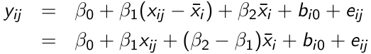
β1 can be interpreted as a purely within-subject (or longitudinal) effect and β2 as between-subject (or cross-sectional) effect. A test of the null hypothesis β1 = β2 is equivalent to the Durbin-Wu-Hausman test for exogeneity.
Linear Fixed Effects Models
Fixed effects linear models are formulated as:
where X denotes a q*1 vector of time-varying covariates, Wi denotes a (p-q)*1 vector of time-invariant covariates and αi are fixed effects representing the time-invariant unobserved confounders, and eij remains the random within-subject errors.
This accounts for all observed/unobserved time-invariate confounders*, making this a model likely less prone to bias with the obvious drawback of way more terms to estimate (loss of power/degrees of freedom)
*assuming that the effects on the response remain constant over time
Although this looks very similar to the random intercepts model considered last class, note that in the mixed effects formulation αi are considered random while now they are considered fixed.
Properties of Fixed Effect Models
- Xij is assumed to be strictly exogenous; i.e. current values of the response Yij given Xij do not predict the subsequent value of Xij+1
- The fixed effects αi can be correlated with Xij and Wi unlike mixed effects where αi are assumed independent of Xij and Wi
- Fixed effects models cannot estimate the effects of time-invariant covariates. Since αi and W'iγ are perfectly colinear, the time-invariant covariates are effectively removed from the analysis
- Fixed effects models remove bias when there are unmeasured but stable characteristics of the subjects that are correlated with time-varying covariates of main scientific interest
Bias-Variance Trade-Off
Although, under the conditions we discussed the fixed effects model may provide unbiased estimates of the time-varying covariates, they will generally have larger standard errors for those estimated effects than those produced by mixed effects models
Fixed effects base estimation exclusively on the within-subject variation and ignore any between-subject variation, while mixed effects utilize both sources of variability resulting in smaller standard errors.
The greater the proportion of between subject variation in a time-varying covariate, the larger the differences in the magnitudes of the standard errors between mixed and fixed effects models.
Comparison of Fixed and Mixed Effects Estimates
Consider the simple random effect model:![]()
It can be shown that the random effects estimator β̂2 RE can be written as: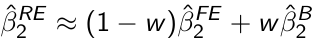
Where β̂2 FE is the fixed effects estimator and β̂2 B is an estimator based only on between-subject variation and is obtained from the regression of Ȳi on X̄i. w is the weight given by: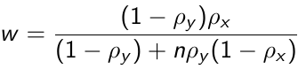
Where ![]() is the proportion of variability in the response due to between subject variation and ρx is the corresponding proportion of variability of Xij that is due to between-subject variation.
is the proportion of variability in the response due to between subject variation and ρx is the corresponding proportion of variability of Xij that is due to between-subject variation.
- When within-subject variation in the response is small then ρy -> 1 which results to w -> 0 and β̂2 RE = β̂2 FE
- When within-subject variation in the covariate is large then ρx -> 1 which results to w -> 0 and β̂2 RE = β̂2 FE
Residual Analyses and Diagnostics
We define a vector of residuals for each individual as ri = Yi - Xiβ̂
From there a simple scatter plot of the residuals against the predicted mean response or covariates can be observed to see if there are is systemic pattern. The residuals are correlated and usually do not have constant variance.
The standardized residuals are defined as: r*i =Li-1ri where Li is a lower triangular matrix so that:
Effectively a Li is a 'square root' [but for matrices] of the var/covar matrix.
ri are uncorrelated and have unit variance. r*ik is an estimate of: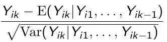
We can use the standardized residuals to detect outlying observations:
- Scatterplot of standardized residuals against teh predicted means response
- Scatterplot of standardized residuals against covariates
- Normal QQ plot to assess the assumption of normallity
- Compute Mahalanobis distance to detect outlying individuals:

di ~ chi-square distributed with degrees of freedom equal to the number of measurements for individual i
Semi-Variogram
We use the semi-variogram to assess the adequacy of a selected model for the covariance.![]()
Where hijk = the time elapsed between repeated measurement j and k on the ith individual. Since E(rij) = 0 then: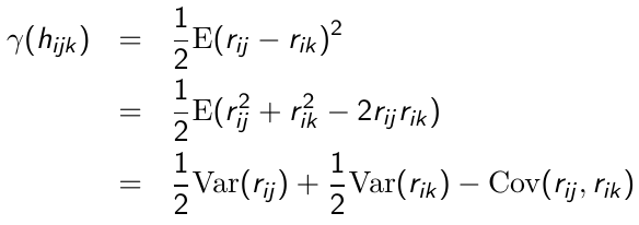
So since each r* has a variance of 1 and covariance of 0, the semi-variogram for r*ij is:![]()
Thus, in a correctly specified model for the covariance the plot of the semi-variogram for the standardized residuals vs. time should fluctuate randomly around a horizontal line centered at 1.
Model Selection Strategy
We can use the following guidelines for selecting a model for correlated data:
- Fit a saturated model such as profile analysis
- For a full model select an appropriate covariance structure using REML. You can use likelihood ratio when appropriate, or AIC/BIC when LRT is not possible
- For an appropriate covariance structure, select an appropriate set of covariates using ML. As previously seen, use LRT, AIC or BIC
- For an appropriate set of covariates, select an appropriate covariance structure using REML
- Repeat steps 3 and 4
Note that REML is used to compare covariance structures to ensure unbiased estimators, ML is used to compare different combinations of covariates because it's more powerful.
SAS Code
/************************************************
* Six cities study of air pollution and health  *
*************************************************/
data fev1;
set s857.fev1;
lgfevht=Log_FEV1_-2*logHgt;
run;

*Durbin-Wu-Hausman test;
*Computes mean age by ID, spits it into another dataset;
proc means data=fev1 ;
*where id ne 197;
by id;
var age ;
output out=mean_age;
run;
data mean_age;
set mean_age;
if _STAT_='MEAN' then;else delete;
rename age=age_mean;
keep id age;
run;
data fev1;
merge fev1 mean_age;
by id;
run;
data fev1;
set fev1;
*Creating mean-centered age;
*Prevents confounding with random slope;
age_dev=age-age_mean;
run;
proc means data=fev1 mean var;
var age age_dev;
run;
proc means data=mean_age;
var age_mean;
run;

*RE model;
proc mixed data=fev1 method=ml covtest;
*where id ne 197;
class id;
model lgfevht=age age_mean/s chisq;
random intercept/type=un subject=id G V ;
run;
*Fixed Effects model;
proc glm data=fev1;
*where id ne 197;
class id;
model lgfevht=id age/solution;
run;
quit;
proc mixed data=fev1 method=ml covtest;
*where id ne 197;
class id;
model lgfevht=age /s chisq;
random intercept/type=un subject=id G V;
run;

*To compute rho of Y (the proportion due to within-subject variation in the repsonse;
*Sigma2(b) is UN(1, 1) = 0.01144, Sigma2(e) is Residual = 0.01391;
proc mixed data=fev1 method=ml covtest;
*where id ne 197;
class id;
model lgfevht=/s chisq;
random intercept/type=un subject=id G V ;
run;
proc mixed data=fev1 method=ml covtest;
*where id ne 197;
class id;
model age=/s chisq;
random intercept/type=un subject=id G V ;
run;
/************************************************
Study of influence of menarche on changes in body fat
*************************************************/

proc sgplot data=s857.fat  noautolegend ;
   * spaghetti plot;
   yaxis min = 0 max = 50;
   reg x=time_men y=Perc_BF
    / group = id nomarkers LINEATTRS = (COLOR= gray PATTERN = 1 THICKNESS = 1) ;
   * overall spline;
   reg x=time_men y=Perc_BF
    / nomarkers LINEATTRS = (COLOR= red PATTERN = 1 THICKNESS = 3) ;
run;
quit;

ods graphics on;

proc loess data=s857.fat plots=all;
   model Perc_BF = time_men;
run;
ods graphics off;

data fat;
set s857.fat;
knot=max(time_men,0);
run;
ods graphics;
proc mixed data=fat covtest plots=all;
model Perc_BF = time_men knot/s chisq outpred=yhat outpm = pred1f residual;
random intercept time_men knot/type=un subject=id G V ;
run;

/*****************************************
*     Mahalanobis Distance          *
*******************************************/
data pred1f;
set pred1f;
sqStudentResid=StudentResid**2;
visits=1;
run;
proc means data=pred1f noprint;
*sum command gives sums in order given (sum of sqStudentResid is output as distance, visits as novisits);
var sqStudentResid visits;
output out=mahalanobis (drop=_type_ _freq_)
sum(sqStudentResid visits)=distance novisits;
by id;
run;
data mahalanobis;
set mahalanobis;
pvalue=1-probchi(distance,novisits);
run;
proc print data=mahalanobis;
*Bonferroni correction to p value based on number of tests;
where pvalue<0.05/162;
run;
/*****************************************/

proc means data=fat;
var time_men;
run;
proc variogram data=pred1f outv=outv noprint;
*Computing measurement differences within subjects with measurement differences (i.e., when they were taken) of up to 10 with iterative values of 1;
*first plot (fit plot) shows average within-subject residuals for different lags. Should be randomly distributed around 0, but def shouldn't have a pattern;

compute lagd=1 maxlag=10;
coord xc=time_men yc=visits;
by id;
var StudentResid;
run;
ods graphics on;

proc loess data=outv plots=all;
   model variog = distance;
run;
ods graphics off;


/*ALternative model*/
data fat;
set fat;
t=time_men;

run;
*Outpred gives FE (population-level) predictions, and outpm gives subject-level predictions;
proc mixed data=fat covtest plots=all;
class t;
model Perc_BF = time_men knot/s chisq outpred=yhat2 outpm = pred2f residual;
random intercept time_men knot/type=un subject=id G V;
*The added repeated statement assumes the error terms don't have constant variances and is looking for that structure;
repeated t/type=sp(exp)(t) subject=id;
run;
data pred2f;
set pred2f;
sqStudentResid=StudentResid**2;
visits=1;
run;
proc variogram data=pred2f outv=outv2 noprint;
compute lagd=1 maxlag=10;
coord xc=time_men yc=visits;
by id;
var StudentResid;
run;
ods graphics on;

proc loess data=outv2 plots=all;
   model variog = distance;
run;
ods graphics off;
Marginal Methods
In many biomedical applications outcomes are binary, ordinal or a count. In such cases we consider extension of generalized linear models for analyzing discrete longitudinal data. These non-linear models require that a linear transformation of the mean response can be modeled in a regression setting. The non-linearity raises issues with the interpretation of the regression coefficients.
We let Yi denote the response variable for the ith subject, and: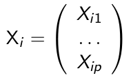
is a p*1 vector of covariates. A generalized linear model for for Yi needs the following three-part specification:
1. A Distributional Assumption
Generalized linear models assume that the response variable has a probability distribution belonging to the exponential family (normal, bernoulli, binomial or Poisson). A feature of the exponential family is the variance can be expressed as:![]()
Where phi is a dispersion parameter and v(μi) is the variance function. For example:
- Variance function of normal distribution: v(μ) = 1
- Variance function of Bernoulli: v(μ) = μ(1 - μ)
2. A Link Function
The link function g(.) applies to the mean and then links the covariates to the transformed mean η such that:![]()
For example, the canonical link functions for some common distributions are: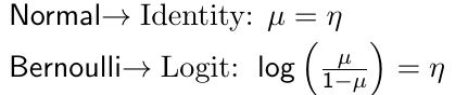
3. A Systematic Component
The systematic component specifies the effects of the covariates Xi on the mean of Yi can be expressed in terms of the following linear predictor:![]()
Note that the term 'linear' refers to the regression parameters.
Binary response
Let Yi denote a binary response variable with two categories such as presence or absence of a disease. The probability distribution is Bernoulli with Pr(Yi = 1) = μi and Pr(Yi = 0) = (1 - μi). Using the logit as the link function we have:![]()
Where μi / (1 - μi) are the odds of success
A unit change of Xik changes the odds of success multiplicitively by a factor of exp(βk).
The logistic regression model can be derived from the notion of a latent variable model. Suppose that Li is a latent continuous variable which follows a standard logistic distribution (0, π2/3) and that a positive response is observed only when Li exceeds some threshold τ , such that:![]()
It can be shown that: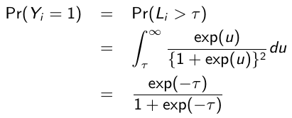
Marginal Models
Suppose Y'i = (Yi1, Yi2 ..., Yip), a vector of correlated responses from the ith subject. To analyze such correlated data we must specify or make assumptions about the multivariate or joint distribution, and to do so we will consider these main extensions of GLM: Marginal Models and Mixed Effects Models (next lecture)
A marginal model for longitudinal data has the following three-part specification:
- E(Yij | Xij) = μij is assumed to depend on the covariates through a known link function:

- We also identify a known variance function:

Where phi is a scale parameter that may be constant or may vary at each measurement occasion. - The conditional within-subject association among the response measurements, given the covariates, is assumed to be a function of an additional set of association parameters, α.
Note that the systematic component is the key building block of a marginal model and specifies the model for the mean response at each occasion, E(Yij | Xij), and its dependence on the covariates. Marginal responses also assume that the conditional mean of the jth response given Xi1, ..., Xin depends only on Xij:![]()
With time-invariant or fixed time-varying covariates this assumption holds. It does not hold when a time-varying covariate varies randomly over time.
Note on association: We avoid using the term correlation. This is because 1) correlation is not a natural measure of within-subject association for discrete responses, and 2) the joint distribution of discrete responses is not often well specified or not easily tractable.
Generalized Estimating Equation
Since there is no convenient or natural specification of the joint multivariate distribution of Yi for marginal models when the responses are discrete, we need an alternative to the Maximum Likelihood estimation. In 1986 Liang and Zeger proposed such a method based on the concept of 'estimating equations' which provides a general and unified approach for analyzing discrete and continuous responses with marginal models. For linear models Generalized Least Sqaures is a special case of estimating equations, for non-linear models the approach is called Generalized Estimating Equations (GEE).
Given a model for the pairwise correlations, the covariance matrix can be expressed as: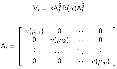
And R(α) is the correlation matrix. Vi is known as a working covariance matrix to distinguish it from the true underlying covariance matrix.
Generalized Estimating Equations
An estimate of β can be obtained as the solution of the following generalized estimating equations: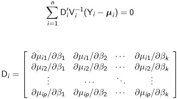
Di can be thought of as a matrix that transforms from the original units of μij to the units of g(μij)
The generalized estimating equations are functions of both β and α and in general have no closed-form solution. In this case, the following two-stage estimation procedure is required:
- Given current estimates of α and φ, Vi is estimated and an updated estimate of β is obtained as the solution of GEE
- Given the current estimate of β updated estimates of α and φ are obtained based on the standardized residuals:

For example, φ can be estimated by: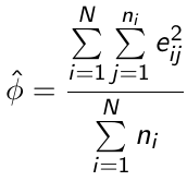
α can be estimated in a similar way:
And steps 1 and 2 are repeated until convergence
Properties of GEE Estimators
β̂_hat is a consistent estimate of β̂, with very high probability and sufficiently large N then β̂_hat ~= β̂. The consistency of β̂_hat depends on the correct specification off the mean, but it still holds even if the covariance of Yi has been mispecified.
By replacing Di, Vi, and sigma_i by their estimates, we get the empirical or sandwich estimator. Note that if we model Vi correctly then Vi = Sigma_i and Var(β̂) = B-1
Daignostics
We can easily calculate residuals:![]()
Since Var(rij) = f(μij) it is preferable to use studentized residuals:
where hij is the leverage of the jth observation on the ith individual and describes the influence each observation has on its own predicted value
We can use diagnostic plots similar to the continuous case to find outlying observations; such as the Mahalonobis-type statistic: 
which has a chi-squared distribution if the model for the mean is correctly specified and Vi ~= sigma_i
SAS Code
* No repeated measures, logistic regression, uses maximum likelihood;
proc logistic data=s857.BPD plots=EFFECT descending;
class BPD;
model BPD=Weight;
title1 'Simple Logistic Regression using PROC LOGISTIC';
run;

* Use GEE, can use if no repeated measures, interpret estimate, never use genmod in non-repeated measures, just here as intro;
proc genmod data=s857.BPD descending;
class BPD;
model BPD=Weight/DIST=binomial LINK=LOGit;
title1 'Simple Logistic Regression using PROC GENMOD';
run;

proc logistic data=s857.BPD plots=EFFECT descending;
class BPD;
model BPD=Weight  Gest_Age Toxemia;
title1 'Multiple Logistic Regression using PROC LOGISTIC';
run;

*Repeated measures, y = obesity;
proc genmod data=s857.BPD descending;
class BPD;
model BPD=Weight  Gest_Age Toxemia/DIST=BINOMIAL LINK=LOGIT;
title1 'Multiple Logistic Regression using PROC GENMOD';
run;
title1 'Marginal Logistic Regression Model for Obesity';
title2 'Muscatine Coronary Risk Factor Study';

*have increase in prevalence in obesity from 8 to 12 then becoems constant for both genders;
*repeated measures since each person has 4 binary measures (obesity status at 4 ages);
proc freq data=s857.muscatine;
where occasion=2;
by gender;
tables age*y;
run;

*apply quad or cubic model since trend not linear;
* 12 is pop mean, dont want multicollinearity when using quad or cubic in model;
* may use these in the model;
data muscatine;
set s857.muscatine;
cage=age - 12;
cage2=cage*cage;
cage3=cage2*cage;
run;

*quad model with respect to age;
* use repeated statement by id (ppl have mult measurements), that variable should also be in class statement;
*type = compund symmetry, so R(alpha) = [1 p p .. p, p 1 p p, p p 1 p...];
/*using a compound symmetry structure working correlation*/
proc genmod data=muscatine ;
     class id occasion;
     model y(event='1')=gender cage cage2 / dist=bin link=logit
     type3 wald;
     repeated subject=id / type=cs  corrw covb;
run;
*look at Analysis of GEE Parameter Estimates table, need to exp estimate if want OR;
*corr parameter is 0.54 from output, no clear interpretation;

/*Using Log OR correlation structure*/
*use logor structure, fullclust says go and find all the associations btwn all the different measures (subj have at most 3 diff measurements) 1&3,1&2,2&3;
proc genmod data=muscatine ;
     class id occasion;
     model y(event='1')=gender cage cage2 / dist=bin link=logit
     type3 wald;
     repeated subject=id / withinsubject=occasion logor=fullclust;
run;
*look at Analysis of GEE Parameter Estimates table;
*three alphas;
*alpha1 = logOR(Yi1, Yi2), OR(Yi1, Yi2) = P(Yi1 = 1, Yi2 = 1)*P(Yi1 = 0, Yi2 = 0) / (P(Yi1 = 1, Yi2 = 0)*P(Yi1 = 0, Yi2 = 1));
* to find OR exp estimate, is OR of having same outcome in occasion 1 and occasion 2 vs diff outcome;
* alpha2 = logOR(Yi1, Yi2);
* alpha3 = logOR(Yi2, Yi3);

*1,2 and 2,3 are only two years apart;
* maybe want alpha1 = logOR(Yi1, Yi2) = logOR(Yi2, Yi3);

/*Equivalent model*/
* three columns, three alphas;
*first row: for 1 2, this is only alpha1;
*second row: for 1 3, this is only alpha2;
*third row: for 2 3, this is only alpha3;
proc genmod data=muscatine descending;
     class id occasion;
     model y=gender cage cage2 / dist=bin link=logit
     type3 wald;
     repeated subject=id / withinsubject=occasion
         logor=zrep( (1 2) 1 0 0,
                     (1 3) 0 1 0,
                     (2 3) 0 0 1) ;
run;

/*The same association between any two occasions */
* compound symmetry but with logOR presentation;
* only one alpha that is same for (1 2) (1 3) (2 3);
* this parametirazation works if same measurement on same subjects at same time (i.e. age 8, 10, 12 for all) like clinical trial design;
proc genmod data=muscatine descending;
     class id occasion;
     model y=gender cage cage2 / dist=bin link=logit
     type3 wald;
     repeated subject=id / withinsubject=occasion
         logor=zrep( (1 2) 1  ,
                     (1 3) 1  ,
                     (2 3) 1 );
run;

/*Testing whether the association between occasions 1-2
and 2-3 are the same */
* three columns, three alphas;
*first row: for 1 2, this is only alpha1;
*second row: for 1 3, this is only alpha2;
*third row: for 2 3, this is alpha1 + alpha3;
* if alpha3 is zero, then (1 2) is same as (2 3), get rid and only have 2 alphas;
proc genmod data=muscatine descending;
     class id occasion;
     model y=gender cage cage2 / dist=bin link=logit
     type3 wald;
     repeated subject=id / withinsubject=occasion
         logor=zrep( (1 2) 1 0 0,
                     (1 3) 0 1 0,
                     (2 3) 1 0 1) ;
run;

/*Fitting a model with the association between occasions 1-2
and 2-3 are the same */
* store p1 = sotre residuals;
proc genmod data=muscatine descending;
     class id occasion;
     model y=gender cage cage2 / dist=bin link=logit
     type3 wald;
     repeated subject=id / withinsubject=occasion
         logor=zrep( (1 2) 1 0 ,
                     (1 3) 0 1,
                     (2 3) 1 0);
store p1;
run;

* plot predicted values for prevalence for diff genders at diff age for quad model;
ods html style=journal;
proc plm source=p1;
  score data = muscatine out=pred /ilink;
run;
proc sort data = pred;
  by gender age;
run;
proc sgplot data = pred;
  series x = age y = predicted /group=gender;
run;

/*Cubic Model*/
proc genmod data=muscatine descending;
     class id occasion;
     model y=gender cage cage2 cage3/ dist=bin link=logit
     type3 wald;
     repeated subject=id / withinsubject=occasion
	 logor=	   zrep( (1 2) 1 0,
                     (1 3) 0 1,
                     (2 3) 1 0);
store p1;
run;

ods html style=journal;
proc plm source=p1;
  score data = muscatine out=pred /ilink;
run;
proc sort data = pred;
  by gender age;
run;
proc sgplot data = pred;
  series x = age y = predicted /group=gender;
run;

/* Example of a quadratic model with gender age interaction */
proc genmod data=muscatine descending;
     class id occasion gender ;
     model y=gender cage cage2 gender*cage gender*cage2  / dist=bin link=logit
     type3 wald;
     contrast 'Age X Gender Interaction' gender*cage 1 -1, gender*cage2 1 -1 /wald;
     repeated subject=id / withinsubject=occasion logor=fullclust;
run;

/*********************************
Diagnostics(Optional)
*********************************/
*assess statement = uses bootstrap to look at sum of residuals, should be centered around 0;
proc genmod data=muscatine descending;
     class id occasion;
     model y=gender cage cage2 cage3/ dist=bin link=logit
     type3 wald;
     repeated subject=id / withinsubject=occasion
         logor=zrep( (1 2) 1 0,
                     (1 3) 0 1,
                     (2 3) 1 0);
	 assess var=(cage)/resamples=10000 seed=7435865;
run;
ods rtf close;
Generalized Linear Mixed Effects Models
Generalized Linear Mixed Models (GLMMs) are an extension of linear mixed models to allow response variables from different distributions (such as binary or multi-nomial responses). Think of it as an extension of generalized linear models (e.g. logistic regression) to include both fixed and random effects.
- The general form of the model is: yij = Xij β + Zij bi + ε
- y (or sometimes η) is a N*1 column vector of the dependent (outcome) variable
- X is a N*p of the p predictor variables
- Z is the N*q design matrix for q random effects (the random complement to the fixed X)
- b (or sometimes u) is a q*1 vector of the random effects
- ε is an N*1 column of vector of the residuals (the part not explained by Xβ + Zu)
- y (or sometimes η) is a N*1 column vector of the dependent (outcome) variable
In classical statistics we do not actually estimate the vector of random effects; we nearly always assume that for the jth element of vector uj ~ N(0, G); Where G is the variance-covariance matrix of the random effects. Recall that the variance-covariance is always square, symmetric and positive semi-definite; This means for a q*q matrix there are q(q+1)/2 unique elements.
Because we directly estimated the fixed effects the random effect complements (Z) are modeled as deviations from the fixed effects with mean 0. The random effects are just deviations around the value in β (which is the mean). The only thing left to estimate is the variance. In a model with only a random intercept G is a 1*1 matrix (the variance of the random intercept). If we had a random intercept and a slope G would look like: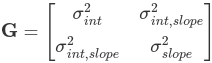
So far everything we've covered applied to both linear mixed models and generalized linear mixed models. What's different about these is that in GLMM the response variables can come from different distributions besides Gaussian. Additionally, rather than modeling the responses directly some link function (referred toi as g(.) and its inverse as h()) is often applied, such as log link. For example, in count outcomes are a special case in which we use a log link function and the probability mass function: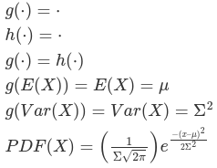
Interpretation
The interpretation of GLMMs is similar to GLMs. Often we want to transform our results to the original rather than the link function result; this is where transformations complicate matters because they are nonlinear and so even random intercepts no longer. Consider the example below of a mixed effects logistic model predicting remission:
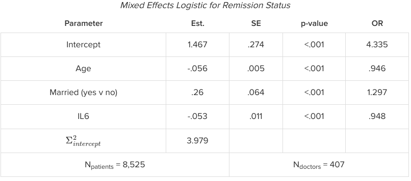
The estimates can be interpreted as always, where the estimated effect of the parameter is interpreted as a change in the log odds. However, we run into issues trying to interpret the odds ratios. Odds ratios take on a more complex meaning when there are mixed effects, as in a regular logistic model we assume all other effects are fixed. Thus we must interpret the odds ratio here as a conditional odds ratio for holding the remaining factors constant.
Estimation
For parameter estimation, there are no closed form solutions for GLMMs you must use some approximation
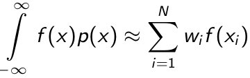
- Gaussian quadrature is a particularly well-suited method to numerically evaluate integrals against probability measures.
- Suppose we have a probability density function p(x) and the function to be integrated against it f(x), the quadrature rule:
where N denotes the number of quadrature points where w is the quadrature weights and x is the abscissas (locations).
- The Gaussian quadrature chooses abscissas in areas of high density, and if it is continuous the quadrille rule is exact is f(x) is a polynomial of up to degree 2R - 1
- In the generalized linear mixed model the roles of f(x) and p(x) are played by the conditional distribution of the data given by the random effects and random effects distribution
- Quadrature abscissas and weights are those of the standard Gauss-Hermite Quadrature
- Suppose we have a probability density function p(x) and the function to be integrated against it f(x), the quadrature rule:
- Gauss-Hermite Quadrature is appropriate when the density is:

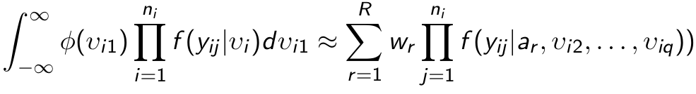
- First we change the variables of integration to independent standard normal random effects v using the Cholesky decomposition L such that G = LL' so that bi = Lvi; We re-write the log likelihood:
where phi(.) is the univariate standard normal density.
- Each uni-dimensional integral can be approximated by Gauss-Hermite quadrature as:
where sqrt(pi)*wr and ar/sqrt(2) are the weights and abscissas of the (2R-1)th degree Gauss-Hermite quadrature rule
- The approximation becomes more accurate as more quadrature points R are used.
- This can be computationally expensive since the number of terms required to evaluate each multivariate integral is Rq
- First we change the variables of integration to independent standard normal random effects v using the Cholesky decomposition L such that G = LL' so that bi = Lvi; We re-write the log likelihood:

Gauss-Hermite quadrature has limitations; The number of function evaluations required grows exponentially as the number of dimensions increases. A random intercept is one dimension, adding a random slope would be two. For three level models with random intercepts and slopes, it is easy to create problems that are intractable with Gaussian quadrature. Consequently, it is a useful method when a high degree of accuracy is desired but performs poorly in high dimensional spaces, for large datasets, or if speed is a concern. Additionally, if the outcome is skewed there can also be problems with the random effects.
SAS Code
libname S857 'Z:\';

data amenorrhea;
set s857.amenorrhea;
t=time;
time2=time**2;
run;

proc sort data=amenorrhea;
by descending trt;
run;
title1 'Marginal Models';
title2 'Clinical Trial of Contracepting Women';

proc genmod data=amenorrhea descending;
class id trt (ref='0') t/param=ref;
model y = time time2 trt*time trt*time2 /dist=binomial link=logit type3 wald;
     repeated subject=id / withinsubject=t logor=fullclust;
store p1;
run;
ods graphics on;
ods html style=journal;
proc plm source=p1;
  score data = amenorrhea out=pred /ilink;
run;
proc sort data = pred;
  by trt time;
run;
proc sgplot data = pred;
  series x = time y = predicted /group=trt;
run;
ods graphics off;

title1 'Generalized Linear Mixed Effects Models';

proc glimmix  data=amenorrhea  method=quad(qpoints=5) empirical order=data ;
class id trt ;
model y = time time2 trt*time trt*time2 /dist=binomial link=logit s oddsratio;
random intercept time/subject=id type=un;
run;

title1 'Generalized Linear Mixed Effects Models';
title2 'Clinical Trial of AntiEpileptic-Drug';
data epilepsy;
set s857.epilepsy;
time=0;y=y0;output;
time=1;y=y1;output;
time=2;y=y3;output;
time=3;y=y3;output;
time=4;y=y4;output;
drop y0 y1 y2 y3 y4;
run;
data epilepsy;
set epilepsy;
if time=0 then t=log(8);
else t=log(2);
run;
proc sort data=epilepsy;
by descending trt;
run;
proc glimmix  data=epilepsy  method=quad(qpoints=50) empirical order=data ;
class id trt ;
model y = time trt trt*time /dist=poisson link=log s offset=t;
random intercept time/subject=id type=un;
run;
ods rtf close;
Multi-Level Modeling
Recall the core of mixed models is that they incorporate fixed and random effects. While single level models assume one variance, subjects within the same level are correlated in terms of σ0j2 + σ1j2Xij + εij
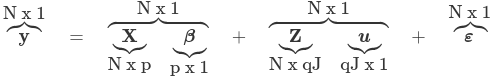
Where y is an N*1 column vector of the outcome
X is a N*p matrix of the p predictors
β is a p*1 matrix of the fixed effects regression coefficents
Z is the N*qJ design matrix for the random effects and J clusters and q random effects
u is a qJ*q vector of q random effects for J clusters/high-level units
Two Level Multi-Level Modeling
MLM is designed to account for hierarchical or clustered structured data. It is especially useful when the "assumption of independence" is violated. Ex. patients by the same doctor, since patients with the same doctor might be more similar.
Using MLMs we can account for repeated measures nested within the individual unit of analysis, as well as comparing units in one 'cluster' to another.
There are multiple ways to deal with hierarchical data. A simple approach is to aggregate, for example if 10 patients are sampled from each doctor we could take the average of all patients within a doctor rather than using individual patients' data. This would lead to consistent effect estimates and standard errors, but it does not really take advantage of all the data so we lose power.
Another approach is to analyze data from one high-level unit at a time, coming up with a regression model for every cluster. But again this does not make full use of the data.
The individual regressions have many estimates and lots of data but is noisy, and the aggregate method is less noisy but loses important differences by averaging all samples within each doctor. Linear mixed models (also called multi-level models) can be thought of as a trade off between these two alternatives.
Random Effects
Random effects capture cluster variability, but they can only exist for a lower level variable. There must be at least one random effect for it to be a multilevel model (but not all random effects have to be included). Typically the intercept is random, which can be thought of as everyone having a slightly different mean adjusted for no other factors. Models with overly complicated random effects may not converge.
As for choosing the structure of the random effects, the most common are unstructured (un) and variance components (VC, this is the default in SAS). So usually the best practice is to try different structures and observe the model fit, but sometimes specifying this structure is not necessary.
Three Level Multi-Level Models
An example of three level data might be schools/classrooms/students. Everything that applies to 2-level models applies to 3-level models as well. These models can have random effects for the 2nd and 3rd level, and must be either completely interdependent or non-interdependent; this requires analysis.
SAS Code
Below is sample SAS code for a campus survey with random effects for ID and campus; In this case the data is nested both within the individual and the campus:
proc mixed data=Final covtest;
class Fake_ID Fake_Campus
(ref="Atlanta") App_Status Discipline
(ref="Engineering/Computer Sciences") ;
model RUCAGRXPRSPOLI = Fake_Campus
Svy_Yr|App_Status svy_YR|Fake_Campus /solution ;
random intercept / type=vc sub=Fake_ID;
random intercept / type=vc sub=Fake_Campus;
run;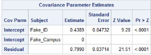
The intercept is the estimate between-subject variance
The residual is the estimated within-subject variance
Effects are significant which means it is okay to include random effects in the model
*2 Level Proc Mixed;
PROC MIXED data=data COVTEST;
CLASS ID;
MODEL DV = Predictor1/CL S DDFM=satterth;
RANDOM INTERCEPT Predictor1 / SUB=ID TYPE=UN;
RUN;

*3 Level Proc Mixed;
PROC MIXED data=data COVTEST;
CLASS DAY ID;
MODEL DV = Predictor1/CL S DDFM=satterth;
RANDOM INTERCEPT Predictor1 / SUB=DAY(ID) TYPE=UN;
RANDOM INTERCEPT Predictor1 / SUB=ID TYPE=UN;
RUN;
Multiple Imputation
If no missing data is present our statistical methods provide valid inference only if the following assumptions are met:
- For Generalized Estimating Equations, the mean function is correctly specified
- For likelihood-based methods, the probability density function including the mean and variance are correctly specified
Missing data can seriously compromise inferences from randomized clinical trials, especially when handled incorrectly, but inference is still possible with the correct methods.
Missing values in longitudinal studies may occur intermittently when individuals miss one or more planned visits, or drop out early.
Types of Missing Data
- Missing Completely at Random (MCAR) - Missingness is independent of both observed and unobserved data. More formally, the probability of missing data in Y is unrelated to the value of Y itself or any other variable X. However, it does allow for the possibility that missingness is Y is related to missingness in some other variable X.
- Ex. In determining predictors of income, MCAR assumption would be violated if people who reported income were on average younger than the people who did report it.
- Missing at Random (MAR) - Missingness is independent of missing responses after controlling for other variables X. Formally: P(Y missing | Y,X) = P(Y missing | X)
- Ex. The MAR assumption is satisfied if the probability of missing data on income depended on a person's age, but within each age group the probability of missing income was unrelated to income. Obviously, this cannot be tested as we do not know the missing values of the data.
- Missing Not at Random (MNAR) - Missing value depend on unobserved values.
- Ex. High income people are less likely to report their income.
- Also referred to as non-ignorable missing or informative dropout
Multiple Imputation
Imputation is substituting each missing value with a reasonable guess, which can be done using a variety of methods. In multiple imputation, imputed values are drawn from a distribution so they inherently contain some variation. Thus, it addresses shortcomings of single imputation by introducing an additional form of error based on variation in the parameter estimates across imputation called between imputation error. Since this is a simulation-based procedure, the purpose is not to re-create the individual missing values as close as possible to the true ones, but to handle missing data to achieve valid inference.
It involves 3 steps:
- Run an imputation model defined by the chosen variables to create imputed data sets. In other words, the missing values are filled in m times to generate m complete data sets.
- The standard is m = 10
- Choosing the correct model requires considering:
- Which variables have missing values?
- Which has the largest proportion of missing values?
- Are there patterns to the missingness?
- Monotone (dropouts in longitudinal studies) or arbitrary
- Perform an analysis on each of the m completed data sets by using a BY statement in conjunction with an appropriate analytic procedure (MIXED or GENMOD in SAS)
- Parameter estimates, standard errors, etc. should be considered
- The parameter estimates from each imputed data set is combined to get a final set of parameter estimates
Pros: Same properties as ML but removes limitations and can be used with any kind of data or software. When the data is MAR, multiple imputation can lead to consistent, asymptotically efficient and asymptotically normal estimates.
Cons: It is challenging to use successfully. It produces different estimates every time.
Use multiple imputation when:
- When there are covariates associated with the missingness of the response but not normally used in the analysis model.
- Ex. In a clinical trial missingness could be related to a side effect which is not a variable in the analysis
- When there are missing covariates; as likelihood-based methods with incomplete covariates are not normally implemented in statistical software and omitted by default.
- When full likelihood methods are not straightforward as in the case of discrete outcomes where GEE methods are often used, although GEE methods are only valid under MCAR and sometimes MAR
Regression-Based Imputation
Particularly with monotone missingness, we can fit a linear regression model to predict missing values Y.
- Randomly draw from a chi-squared distribution with (Nj - q) degrees of freedom where Nj is the number of subjects who haven't dropped out at the jth occasion and q is the number of covariates used to predict Y.
- Calculate the residual variance of the kth draw:
$$\sigma^2 = (N_j - q) \hat\sigma^2 / \chi^2 $$ - Randomly draw regression parameters γ from a multivariate distribution N(γ, Cov(γ)) where:
$$ Cov(\hat\gamma) = \sigma^2 (\sum_{i=1}^{N_j} Z_{ij} Z'_{ij})^{-1} $$
- Draw e from N(0, σ2), where σ2 is the estimate of residual variance
- Calculate Yij = Z'ijγ + e
- Repeat 1-5 m times
Predictive Mean Matching
This method is very similar to regression based imputation. This is more robust against misspecification of the regression model and ensures all imputed values are plausible.
- See step 1 above
- See step 2 above
- See step 3 above
- Calculate Yij = Z'ijγ
- Select a subset of K observations whose predicted values are closest to Yij
- Impute the missing value by randomly drawing from these K observed values
- Repeat step 1-6 m times.
Bayesian Principals of Imputation
\(Y^{obs} \) = Observed (vector of) quantities
\(Y^{mis} \) = Missing (vector of) quantities
\( \theta \) = Parameter of interest (unobserved)
R = Indicator variable which takes the value 1 for observed part of Y and 0 elsewhere (observed)
\( \tau \) = Parameter (vector) to describe missing data mechanism (unobserved)
Assume our data has a prior distribution: \( \pi(Y_i | X_i, \tau ) \) where \( \tau = (\beta, \theta) \)
The predictive posterior:
\(\pi( Y^{mis}_i | Y^{obs}_i, X_i ) = \int \pi(Y^{mis}_i | Y^{obs}_i, X_i, \tau) \pi(\tau | Y^{obs}_i, X_i ) d\tau \)
And the observed-data posterior is closely related:
\(\pi( \tau | Y^{obs}_i, X_i ) = \int \pi( \tau | Y^{obs}_i, Y^{mis}_i, X_i) \pi(Y^{mis}_i | Y^{obs}_i, X_i ) dY_{mis}
= E_{Y^{mis}_i | Y^{obs}_i} (\pi(\tau | Y^{obs}_i, Y^{mis}_i, X_i) \)
Markov Chain Monte Carlo for Multiple Imputation
- Imputation step: Given a current estimate \( \hat\tau^k \) of the parameters, first simulate a draw from the conditional predictive distribution of \( Y^{mis^{k + 1}}_i \) conditional on the observed values and tau:
$$ Y^{mis^{k + 1}}_i \sim \pi(Y^{mis}_i | Y^{obs}_i, X_i, \hat\tau^k) $$ - Posterior P-step: Given a complete sample \((Y^{obs^k}_i , Y^{mis^{k+1}}_i)\) take a random draw from the complete-data posterior:
$$ \hat\tau^{k + 1} \sim \pi(\tau | Y^{obs}_i, Y^{mis^{k+1}}_i, X_i) $$ - Repeat these two steps starting from \(\hat\tau^0\), create a Markov chain, {\( \hat\tau^k, Y^{mis^k}_i, k = 1, 2 ... \)} whose stationary distribution is \( \tau, Y^{mis}_i. X_i \) with stationary distributions:
\(\hat\tau^k (k = 1,2,...) \sim \pi(\tau | Y^{obs}_i, X_i )\) and
\(Y^{mis^k}_i (k = 1,2,...) \sim \pi(Y^{mis}_i | Y^{obs}_i, X_i )\)
SAS Code
/*We have created 25 versions of the same dataset
with no missing values. We can run proc mixed
for each version seperately...*/
proc mixed data=MITLC_long;
where _imputation_=2;
class TRT TIME;
model y=time time*trt/s covb;
repeated time/type=un subject=id;
run;

/*
...or run all 25 in one run using a by statement
and saving the solutions using an ods output statement
*/
proc mixed data=MITLC_long;
class TRT TIME;
model y=time time*trt/s covb;
repeated time/type=un subject=id;
by _IMPUTATION_;
ods output solutionf=beta covb=varbeta;
run;

proc mianalyze parms=beta;
class TRT TIME;
modeleffects intercept time TRT*time;
run;

/*Using MCMC for imputation*/
proc sort data=TLC_missing;
by TRT;
run;
proc mi data=TLC_missing seed=364865 nimpute=25 out=miTLC_MCMC;
var y4 y6;
by TRT;
mcmc chain=multiple displayinit initial=em(itprint);
run;

data MITLC_MCMC_long;
set MITLC_MCMC;
y=y0;time=1;OUTPUT;
y=y1;time=2;OUTPUT;
y=y4;time=4;OUTPUT;
y=y6;time=6;OUTPUT;
drop y0 y1 y4 y6;
run;

proc sort data=MITLC_MCMC_long;
by _IMPUTATION_;
run;

proc mixed data=MITLC_MCMC_long;
class TRT TIME;
model y=time time*trt/s covb;
repeated time/type=un subject=id;
by _IMPUTATION_;
ods output solutionf=beta_mcmc covb=varbeta_mcmc;
run;

proc mianalyze parms=beta_mcmc;
class TRT TIME;
modeleffects intercept time TRT*time;
run;
Mutlivariate and Joint Models for Longitudinal Data
Longitudinal studies are commonly designed in many research fields in order to see changes over a time interval shared by all participants. Joint modeling consists of two interlinked sub-models with any type of outcome (continuous, binomial, etc). One of the most commonly used is longitudinal sub-model is the linear mixed effect model and a cox proportional hazard with time-to-event sub-model.
Joint modeling reduces the bias of parameter estimates by accounting for the association between the longitudinal and time-to-event data. In clinical trials this often leads to more efficient estimation of the treatment effect on both sub-model outcomes.
Let's assume Yi1 and Yi2 are two outcomes measured on subject i. We can attempt to specify a joint density f(yi1, yi2), but this is only feasible if we assume certain things about the marginal association among the longitudinally measured elements within each of the outcome vectors. This is easier when both outcomes and conditional models are of the same type, but this is not a requirement. When Yi1 and Yi2 are of different types, or in the case of unbalanced data, this becomes cumbersome. Thus, extensions to higher dimensional data involves considerable challenges as this would require assumption on larger covariance structure and higher order associations.
Conditional Models
We can avoid direct specification of the joint density f(yi1, yi2) are and reduce the modeling tasks by specifying a model for each outcome separately:
f(yi1, yi2) = f(yi1 | yi2) f(yi2)
= f(yi2 | yi1) f(yi1)
The main drawback is that this requires reflection about the plausible association between Yi1 and Yi2 that may be inappropriate in some settings. For example, in a clinical trial with two main post-randomization outcomes conditioning on one of the outcomes may attenuate (make smaller) the treatment effect on the other. Also, it is difficult to implement in high-dimension data.
Shared-Parameter Models
In previous chapters we've seen how random effects can be used to generate an association structure between repeated measurements of a specific outcome. We can use a similar approach to generate association between two outcomes.
\( f(y_{i1}, y_{i2}) = \int f(y_{i1}, y_{i2} | b) f(b) db = \int f(y_{i1} | b) f( y_{i2} | b) f(b) db \)
Where b is a vector of ranom effects common to the outputs Yi1 and Yi2, and assume independence of both outcomes conditional on b.
Again the outcomes do not have to be of the same type, but we assume b represents a common set of unobserved characteristics of the subject that governs both models.
Examples:
Let Yi1 represent a vector of longitudinal continuous outcomes and Yi2 = (Ui, 𝛿i) with U = min(Ti, Ci) with Ti as the potential time to the event of interest, Ci as the potential censoring time, and 𝛿i = I(Ti <= Ci). Let Yi1 follow a random intercept model:
Y = β0 + b0i + β1t + εi1t
and let the event time of interest follow a proportional hazard model so that:
where λ0(t) is an unspecified baseline hazard function
In another case, the shared-parameter random effect models may imply very strong assumptions for the association structure between outcomes. Consider this example where Yi1 and Yi2 are two longitudinal continuous outcomes that share a common random intercept: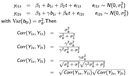
The joint random-effects imply more flexible correlation patterns. Consider this example where Yi1 and Yi2 are dependent on separate random effects b1 and b2 which are themselves correlated: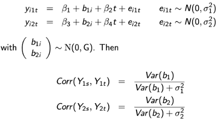
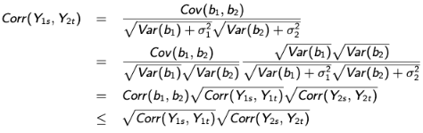
This demonstrates the role of the correlation between the outcome-specific random effects in the between-process outcome correlation at any two time points. The restriction is imposed by the shared-parameter model is relaxed in the same sense that the model no longer assumes the product of within process correlations equals the between-process correlation and thus allows a more general dependence structure.
In many situations (especially when we have multiple outcomes/high-dimensional data) the previous methods will not be feasible to estimate. Methods that reduce the dimensions are more appropriate. The idea is to use a factor-analytic or principal component type of analysis to reduce the dimensions. After, the estimated factors can be analyzed using any of the classical longitudinal models. The disadvantage is that the inferences are restricted to the factors and cannot be extended to the original outcome variables, so certain assumptions need to be imposed in the case of unequally spaced observations or unbalanced designs.
Defining the Generalized Linear Models
For a bi-variate response Yi = (Yi1, Yi2)', we can assume a general model in the form of: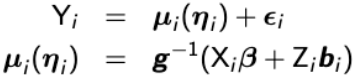
with g-1 as the inverse link function which is allowed to change for each univariate outcome and bi ~ N(0, G).
A general first-order approximate expression for the variance-covariance matrix of Yi is:
Var(Yi) ~= Δi Zi GZ'iΔ'i + Vi
Where 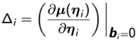 and
and ![]()
and R( α ) is the correlation matrix and the Ξi is a diagonal matrix with over-dispersion parameters along the diagonal: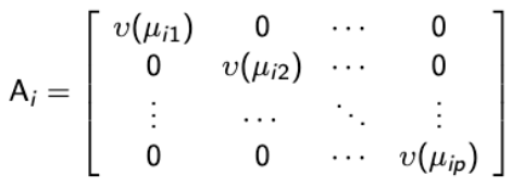
If there are no random effects then the model is referred to as a marginal generalized linear model (MGLM). For the special case of a continuous and binary endpoint the MGLM is in the form of: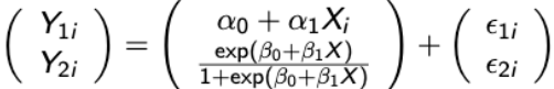
with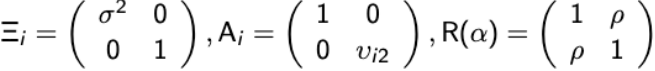
vi2 = μi2(1-μi2)
In a shared parameter the variance of Yi is approximately equal to: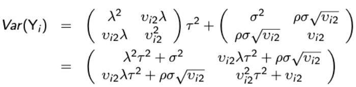
As a result the approximate correlation among the two outcomes is:
The correlation depends on the fixed effects through vi2
SAS Code
libname s857 "/Datasets";
options fmtsearch=(s857.formats);
options nofmterr;

proc mixed data=s857.Tbi;
class sex naccid  status;
model Mem1=time  naccageb status sex time*educ time*naccageb  /solution;
random Int time/sub=naccid;
run;

proc mixed data=s857.Tbi;
class sex naccid  status;
model Att1=time  naccageb status sex time*educ time*naccageb  /solution;
random Int time/sub=naccid;
run;

/* Multivariate models  */
data s857.tbi_long;
length scale $10;
set s857.tbi;
Outcome=Mem1;scale='Memory';output;
Outcome=Att1;scale='Attention';output;
keep Outcome Scale time trauma_dich dep2yrs status sex educ naccageb naccid;
run;
proc mixed data=s857.tbi_long covtest method=ML;
class Scale sex naccid  status;
model Outcome=Scale*time Scale*naccageb Scale*status Scale*time*status
 Scale*sex Scale*time*educ Scale*time*naccageb  /solution;
random Int time/sub=naccid;
*random int/sub=Scale type=un;
run;

proc nlmixed data=s857.tbi_long;
parms b0=-0.17 b1=0.43 b2=0.39 b3=-0.83 b4=0.08 b5=-0.01
s2e_mem=0.361 g11=0.60
	c0=0.05 c1=-0.05 c2=0.5 c3=0.1
s2e_att=0.19;
if Scale='Memory' then do;
	mean=b0+b1*time + b2*status + b3*sex +b4*time*status +b5*time*naccageb  +u1 ;
	ll = -0.5*log(3.14159265358) - log(sqrt(s2e_mem)) -0.5*(outcome-mean)**2/(s2e_mem);
end;
if Scale='Attention' then do;
	mean=c0+c1*time + c2*status + c3*time*status  +u1;
	ll = -0.5*log(3.14159265358) - log(sqrt(s2e_att)) -0.5*(outcome-mean)**2/(s2e_att);
end;
model outcome~general(ll);
random  u1~normal([0],[g11]) subject=naccid;
run;

/*Shared parameter model*/
title 'Memory';
proc mixed data=s857.tbi covtest method=ML;
class trauma_dich sex naccid  status;
model Mem1=time status  sex time*status time*naccageb  /solution;
random intercept/sub=naccid;
run;
title 'Attention';
proc mixed data=s857.tbi covtest method=ML;
class trauma_dich sex naccid  status;
model Att1=time /solution;
random intercept/sub=naccid;
run;

proc nlmixed data=s857.tbi_long;
parms b0=-0.13 b1=0.43 b2=0.39 b3=-0.83 b4=0.08 b5=-0.01
s2e_mem=0.361 g11=0.60
	c0=0.05 c1=-0.05 c2=0.5 c3=0.1 gamma=0.20
s2e_att=0.19;
if Scale='Memory' then do;
	mean=b0+b1*time + b2*status + b3*sex +b4*time*status +b5*time*naccageb  +u1 ;
	ll = -0.5*log(3.14159265358) - log(sqrt(s2e_mem)) -0.5*(outcome-mean)**2/(s2e_mem);
end;
if Scale='Attention' then do;
	mean=c0+c1*time + c2*status + c3*time*status  +gamma*u1;
	ll = -0.5*log(3.14159265358) - log(sqrt(s2e_att)) -0.5*(outcome-mean)**2/(s2e_att);
end;
model outcome~general(ll);
random  u1~normal([0],[g11]) subject=naccid;
run;
proc nlmixed data=s857.tbi_long;
parms b0=-0.13 b1=0.43 b2=0.39 b3=-0.83 b4=0.08 b5=-0.01
s2e_mem=0.361 g11=0.60 g22=.01
	c0=0.05 c1=-0.05  c2=-0.3 c3=-0.1 gamma=1 g33=0.01
s2e_att=0.19;
if Scale='Memory' then do;
	mean=b0+b1*time + b2*status + b3*sex +b4*time*status +b5*time*naccageb  +u1 +u2*time;
	ll = -0.5*log(3.14159265358) - log(sqrt(s2e_mem)) -0.5*(outcome-mean)**2/(s2e_mem);
end;
if Scale='Attention' then do;
	mean=c0+c1*time + c2*status + c3*time*status  +gamma*u1 +u3*time;
	ll = -0.5*log(3.14159265358) - log(sqrt(s2e_att)) -0.5*(outcome-mean)**2/(s2e_att);
end;
model outcome~general(ll);
random  u1 u2 u3~normal([0,0,0],[g11,0,g22,0,0,g33]) subject=naccid;
run;
proc nlmixed data=s857.tbi_long;
parms b0=-0.13 b1=0.43 b2=0.39 b3=-0.83 b4=0.08 b5=-0.01
s2e_mem=0.361 g11=0.60 g22=.01 g12=0.01
	c0=0.05 c1=-0.05  c2=-0.3 c3=-0.1
s2e_att=0.19;
if Scale='Memory' then do;
	mean=b0+b1*time + b2*status + b3*sex +b4*time*status +b5*time*naccageb  +u1 ;
	dens = -0.5*log(3.14159265358) - log(sqrt(s2e_mem)) -0.5*(outcome-mean)**2/(s2e_mem);
	ll=dens;
end;
if Scale='Attention' then do;
	mean=c0+c1*time + c2*status + c3*time*status  +u2;
	dens = -0.5*log(3.14159265358) - log(sqrt(s2e_att)) -0.5*(outcome-mean)**2/(s2e_att);
	ll=dens;
end;
model outcome~general(ll);
random  u1 u2~normal([0,0],[g11,g12,g22]) subject=naccid;
run;

/*
if dist='Binary' then do;
		eta=v0 + v1*u1   ;
		p=exp(eta)/(1+exp(eta));
		ll = (outcome)*log(p) + (1-outcome)*log(1-p);
end;
*/
Time Series Models
While standard regression we must assume observations are independent from one another, but with time series data we expect that neighboring observations are correlated. Time series analysis helps organizations understand the underlying causes of trends or systemic patterns over time. A time series is simply a set of statistics that is collected at regular intervals which we can use too obtain valid inferences. Ex. the daily number of live births or death.
A Single Observation of Stochastic Process
A Stochastic process is a (possibly) infinite sequence of variables ordered in time {Y0, Y1, Y2 ...}. A time series is a single realization of a stochastic process. We want to make inference about the properties of the underlying stochastic process from a single observation.
There are two assumptions in time series analysis:
- The data sequence is stationary. This means if all the times are shifted by the same amount, the probability distribution remains the same; meaning it depends on relative and not absolute values. In other terms:
\( (X_{t_1}, ... , X_{t_k}) =(X_{t_{1 + h}}, ... , X_{t_{k + h}}) \)
for all time points t and integer h
Under this assumption we can use the replication over time to make inferences about the common mean, variance, and other statistics. Additionally, the degree of independence increases as the time interval between two observations increases. - Ergodicity - the ability to make valid probability statements by looking over time rather than across replicates across one time.
Auto-correlation
A consequence of independence when observations are far apart enough in time is that we can use the auto-correlation function as a measure of dependence of the observations over time.
Let us define the covaraiance between time points at lag k as:
\(\gamma(k) = Cov(Y_{k+1}, Y_1) = Cov(Y_{k+2}, Y_2) \)
And from that we can define the autocorrelation function as:
\( \rho(k) = \gamma(k) / \gamma(0) = corr(X_t, X_{t+k}) \)
We can also take a partial autocorrelation which is a conditional correlation. This is the correlation between two variables under the assumption that we know and take into account the values of some other set of variables.
Partial autocorrelation can be imagined as the correlation between the series and its lag, after excluding the contributions from the intermediate lags. So, PACF sort of conveys the pure correlation between a lag and the series. That way, you will know if that lag is needed in the AR term or not.
Auto-regressive Processes
An autoregressive process of order p is denoted by AR(p) is defined by
\( Y_t = \phi_1 Y_{t-1} + \phi_2 Y_{t-2} + ... + \phi_p Y_{t-p} - \epsilon_t \)
with \(\epsilon_t \) ~ N(0, 𝜎2)
Or in other terms:
\( Y_t = \sum_{r=1}^{p} \phi_r Y_{t-r} + \epsilon_t \)
Where phis are a fixed constants
The outcome only depends on its own lags.
Moving Average Process
A time series Yt is called a moving average process of order q (MA(q)) if:
\( Y_t = \sum_q^{s=0} \theta_s \epsilon_{t-s} \)
where thetas are a fixed constraint, theta_0 = 1
The sequence \(\epsilon_t\) consisting of independent random variables with mean 0 and variance \(\sigma^2\) are called white noise. It is a second order stationary series with \(\gamma_0 = \sigma^2 \) and \(\gamma_k = 0 \) for k != 0
The outcome depends only on the lagged forecast errors.
ARMA Models
ARIMA, short for ‘Auto Regressive Integrated Moving Average’ is actually a class of models that ‘explains’ a given time series based on its own past values, that is, its own lags and the lagged forecast errors, so that equation can be used to forecast future values.
An ARIMA model is characterized by 3 terms: p, d, q
- p is the order of the AR term; It refers to the number of lags of Y to be used as predictors.
- q is the order of the MA term; the number of lagged forecast errors that should go into the ARIMA Model.
- d is the number of differencing required to make the time series stationary.