Advanced Topics
Post-grad notes on new research techniques
- Propensity Score Weighting Analysis
- Heterogeneous Graph Learning
- Sampling
- Forecasting with Geospacial Data
- Advanced Machine Learning
Propensity Score Weighting Analysis
Unlike randomized clinical trials, observational studies must adjust for differences such as confounding to ensure patient characteristics are comparable across treatment groups. This is frequently addressed through propensity scores (PS), which summarizes differences in patient characteristics between treatment groups. A Propensity Score is the probability that an individual will be assigned to receive the treatment of interest given their measured covariates. Matching or Weighting on the PS is used to adjust comparisons between the 2 groups, thus reducing the potential bias in estimated effects of observational studies.
The following use cases assume a binary treatment or exposure in order to infer causality. Given a treatment and control with one outcome observed per unit, can we estimate the treatment effect? Note we can only estimate the treatment effect, identification of causality is not possible through observational studies.
Note the following definitions before proceeding:
- Target Population - The group of individuals who we wish to infer conclusions about
- Balance - Similarity of patient characteristics across treatment
- Precision - Denotes certainty about the estimate of association between treatment and outcome of interest; More precision means more narrow CIs and greater statistical power.
Estimation of Propensity Scores
Propensity scores are most commonly estimated using binomial regression models (logistic regression, probit, etc.). Other propensity score methods include:
- Classification Trees
- Bagging/Boosting
- Neural Networks
- Recursive Partitioning
Basically, any model that provides predictive probability and where all the covariates related to treatment and outcome that were measured before treatment are included in the propensity score estimation model. The SAS example below estimates propensity scores for the treatment variable group predicted from covariates var1, var2, and var3 using a logistic regression:
PROC LOGISTIC data=ps_est;
  title 'Propensity Score Estimation';
  model exposure = var1-var3 / lackfit outroc = ps_r;
  output out = ps_p pred = ps xbeta=logit_ps;
  /* Output the propensity score and the logit of the propensity score */
run;
Once we have the propensity scores estimated, we must make sure the measured covariates are balanced in order to reduce bias. There are several ways to achieve this:
- Graphic of the propensity score distribution - The distribution of propensity score between the two groups should overlap. Non-overlapping distributions suggest that one or more covariates are strongly predictive, and variable selection or stratification should be reconsidered.
- Standardized differences of each covariate between treatment groups - the magnitude of the difference between baseline characteristics of the groups can be calculated depending on the method of deriving propensity scores. One limitation of this method is the lack of consensus as to what the threshold should be, though researchers have suggested a standardized difference of .1 or more denotes meaningful imbalance in the baseline covariates.
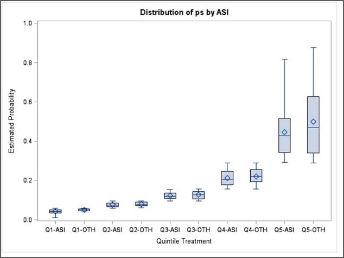
- Stratify by deciles or quintiles (5 parts) - By stratifying the propensity score by deciles or quintiles, a boxplot can represent each quintile.
When the scores aren't balanced, the covariates in the model should be adjusted. This could mean adding or removing covariates, adding interactions, or substituting a non-linear term for a continuous one.
Covarite Balancing Propensity Scores
After we obtain the propensity score, the next step is to estimate the Average Treatment Effect in the population (ATE). Using multiple methods can help strengthen conclusions, while discrepancies can indicate confounding and/or sensitivity to the analysis approach.
A key diagnostic is the standardized mean difference (SMD)- The normalized difference in means between two groups for a given covariate. A SMD score of > .1 for a given covariate generally indicates imbalance.
Stratification
Stratification divides individuals into many groups on the basis of their propensity score values. The optimal number of strata depends on sample size and the amount of overlap between treatment and control group propensity scores, however researchers have suggested 5 subclasses is sufficient enough to remove 90% of bias in the majority of PS studies. The treatment effect for each subclass is the average effect across strata weighted by stratum-specific standard error:
$$ \hat\mu_{1i} - \hat\mu_{2i} = {{\sum w_i (\bar X_{1i} - \bar X_{2i}) } \over {\sum w_i}} $$
Where \( w_i = { 1 \over {SE}^2_i} \) (the square of the standard error of the difference between means). This can be coded in SAS as follows:
/* Stratify */
PROC RANK data=ps_p out=ps_strata groups=5;
	var ps_pred;
    ranks ps_pred_rank;
run;

/* Sort */
proc sort data = ps_strataranks;
	by ps_pred_rank;

/* Compute the difference between group means in each stratum,
	as well as the standard error of this within stratum difference */
proc ttest;
  by ps_pred_rank;
  class group;
  var outcome;
  ods output statistics = strata_out;

/* Find stratum specific weights and mutliply by mean difference */
data weights;
  set strata_out;
  if class = 'Diff (1-2)';
  wt_i = 1/(StdErr**2);
  wt_diff = wt_i*Mean;

/* Find the mean weighted difference and its standard error */
proc means noprint data = weights;
  var wt_i wt_diff;
  output out = total sum = sum_wt sum_diff;
  data total2;
  set total;
  Mean_diff = sum_diff/sum_wt;
  SE_Diff = SQRT(1/sum_wt);

proc print data = total2;

run;
Matching
The goal of matching is to obtain similar groups of treatment and control subjects by matching individual observations on their propensity scores. It is generally recommended to use 1:1 matching with no replacement to avoid bias. The Nearest Neighbor (or Greedy matching) selects a control unit for each treated unit based on the smallest distance from the treated unit. The big problem with this is it depends on the order in which the data is sorted, thus randomization is necessary.
Nearest Neighbor with calipers is a method which improves NN by allowing a maximum allowable difference between scores (or caliper width) in order for PS to be matched. Researchers have suggested a caliper width of .2 times the standard deviation, or a static value such as .1.
The general procedure:
- Sort observations into random order with each group
- Transpose data to obtain seperate datasets for treatment and control
- Merge them into a single dataset, matching each observation in the treatment group with a single observation in the control group
- If no control observations are found in the range, no matched pair is created
- After matched pairs have been identified, the difference in outcome means in each group can be tested ussing a t-test.
- Use a correlated-means t-test rather than independant-means (PAIRED keyword in SAS)
/* Use the propensity score model probabilities to match case and control 1:1 */
proc psmatch data=ps_p region=cs;
  class exposure;
  psmodel exposure = var1-var3;
  match distance=lps method=greedy(k=1) stat=lps caliper(mult=stddev)=.15;
  assess lps var=(var1-var3)/weight=none plots=(boxplot);
  output out(obs=match)=match1 lps=_Lps matchid=_MatchId;
run;
Inverse Probability of Treatment Weights (IPTW)
In IPTW, individuals are weighted by the inverse probability of receiving the treatment they actually received. So, the target estimand is the treatment effect in the treated population. Control subjects are weighted by \(1 / (1 - p_i) \) and treated subjects with \( 1/p_i \). The weights are then used in a Weighted Least Squares regression model.
data ps_weight;
  set ps_p;
  if group = 1 then ps_weight = 1/ps_pred;
  else ps_weight = 1/(1-ps_pred);
run;

proc means noprint data = ps_weight;
  var ps_weight;
  output out = q mean = mn_wt;
run;

data ps_weight2;
  if _n_ = 1 then set q;
  retain mn_wt;
  set ps_weight;
  wt2 = ps_weight/mn_wt; * Normalized weight;
run;

/* Either of the below can be used to estimate treatment effect
 via weighted least sqaures */
proc glm data = ps_weight2;
  class group;
  model outcome = group / ss3 solution;
  weight wt2;
  means group;
run;

proc reg data = ps_weight2;
  model outcome = group;
  weight wt2;
run
The IPTW method is inclusive of all subjects, so no data loss occurs. However, it is very sensitive to outliers and can create extreme weights. There exist stabilization techniques which use trimming or scaling to get weights into a specified range.
Overlap Weighting
Overlap weighting (OW) is a new PS method aimed to address the shortcoming of IPTW. In IPTW, individuals are weighted by the inverse probability of being in their treatment group, which allowed under-representing characteristics to count more. In OW, patients are assigned weights which are proportional to the probability of that patient belonging to the other treatment group. That is, treated patients are given a weight of (1 - PS) while non-treated are weighted by the probability of treatment PS. The target estimand is the average treatment effect for the overlap population.
These weights are smaller for extreme values so outliers are treated as PS near 1 or 0, and do not dominate or worsen precision as with IPTW. Patients whose characteristics are compatible with either group contribute relatively more. The result can be as efficient as randomization. Overlap weighting creates an exact balance on the mean of every measured covariate when the PS is estimated by logistic regression. This is advantageous when groups being compared are initially very different.
We can use the code from IPTW replacing the weight of 1/PS with 1 - PS in the treated group and 1/(1-PS) with PS in the untreated group. Note that adjustments such as trimming have nearly no effect on the weighted balance of OW.
* Generating overlap wieghts;
data overlap;
  set ps_p;
  ow_weight = (EXPOSURE)*(1-ps) + (1 - EXPOSURE)*ps;
run;

* then normalize it;
Estimating Treatment Effect
With the generated weights or matched dataset pick a fitting model to determine the effects of the exposure on the outcome of interest. If any covariates remain imbalanced, they can be included in the model. Otherwise, the model should only contain outcome and exposure.
* Continous Outcome;
proc glm data=overlap2;
  class exposure(ref="0");
  model OUTCOME = EXPOSURE/solution;
  weight ow_weight;
run;

* Dichotomous outcome (in this case coded into several binary variables);
proc genmod data=overlap2;
  class exposure(ref="0");
  model OUTCOME1 = EXPOSURE/dist=BINOMIAL;
  weight ow_weight;
run;
R
The above code examples use SAS to explain the underlying concepts. There are several R packages that can provide propensity score weighting with binary treatments, but the newest and most popular is PSweights. I recommend checking out the documentation and whitepaper (link below) to understand the functionalities this package can provide.
References
Overlap Weighting: A Propensity Score Method That Mimics Attributes of a Randomized Clinical Trials
Propensity Score Analysis and Assessment of propensity Score Approaches Using SAS Procedures
PSweight: An R Package for Propensity Score Weighting Analysis
https://www.r-causal.org/chapters/08-propensity-scores
Heterogeneous Graph Learning
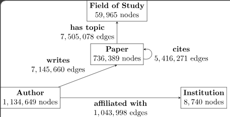
Knowledge graphs are visualization of information with multi-type relations (edges) among some multi-type entities (nodes) within an environment of interest. The heterogeneous aspect comes from the graph having two or more types of nodes and two or more types of edges.
Usage: Alzheimer's Drug Repurposing
In recent studies on Alzheimer's drug repurposing (Reference 1) Graph Neural Networks (GNN) were used to identify biological interactions from prior knowledge databases containing information on effective treatments and genes associated with high risk. The nodes of the graph included drugs, genes, pathways and gene ontology (GO) connected by interactions including drug-target interaction, drug-drug structural similarity, gene-gene interaction, gene-pathway association, gene-GO association and drug-GO association. A comprehensive graph can be created combining existing information from multiple sources on the biological interactions of complex drug-gene relationships, and from there we can use machine learning to train a model and address the incomplete knowledge in the graph. Note that in this paper the genes are encoded/embedded, simply meaning they are represented as numerical vectors/matrices to capture their function. To give a broad overview of the study's workflow:
- A knowledge graph is built to describe the interaction between drugs, genes, gene ontology and pathways
- Node embeddings are derived using a multi-relational Variational Graph Auto-Encoder (VGAE)
- Machine learning model ranks drug-candidates based on multi-level evidence
- Drug combinations are searched for complementary exposure patterns, using previously ranked drug candidates
- Validate drug combinations with "oxidative stress responses" and randomly removing edges to see if the model can correctly predict interactions
By keeping the focus previously approved drugs, the graph can identify synergy between medications that treat complex diseases. The "Complementary Exposure Pattern" of analysis used suggests drug combinations are effective when the target of the drugs hit the disease module without overlap.
While this study breaks ground in applying knowledge graphs with multi-task learning to fragmented multi-modal data, it is subject to the limitations of each dataset it combines. The knowledge graph alone extracts data from:
- 5,874,261 Universal protein-protein interactions from STRING, Drug Bank, HetioNet, GNBR, and IntAct
- Interaction between genes, drugs, GO, and pathways from Comparative Toxicogenomic Database (CTD)
- Drug-Drug associations based on structural similarities using scores from the RDkit package
- Gene IDs from National Center for Biotechnology information (NCBI)
- High confidence Alzheimer's associated genes from Agora's nominated gene list
If any of the data-driven drug efficacy is biased, then so is the model. Some of the datasets contained in vitro studies (lab based experiments usually in a test tube), which does not guarantee identical treatment outcomes. Still, given the lack of clinical evidence from a huge list of compounds, this research could provide insight on drug combinations in future research opportunities.
VGAE
One of the key elements in the knowledge graph is the customized deep Variational Graph neural Auto-Encoder (VGAE), used to incorporate multiple types of relationships (edges). It is a self-supervised technique which encodes the nodes into a latent vector (embedding) and reconstruct the graph with the latent vector. This approach allows the incorporation of the uncertainty of our knowledge of a given node, thus creating a probabilistic distribution. Different weight matrices were also determined for each type of edge.
Within the Alzeimer's drug GNN Pytorch Geometric was used for the model implementation. It was trained to reconstruct missing interactions using the node embeddings as an autoencoding manner. To do this, each node's embedding is iteratively updated by aggregating their neighbors' embedding, in which the average of the neighbors' features are taken, concatenated with the current embedding, and applied to a single layer of a neural network.
Transfer Learning
Transfer learning is to transfer knowledge from previously learned universal models to domain-specific models. Injecting universal knowledge on pharmacological interactions while prioritizing Alzheimer's is a critically important step in identifying uncertainty. The Drug Repurposing Knowledge Graph (DRKG) network was used as the universal data source, containing over 15 million pharmacological entities including 39 different interactions between compounds and genes from various biomedical databases. The pretrained embeddings for drugs, genes, pathways and GOs were used as initial node features and then fine-tuned, but the edges were not always directly incorporated as the interactions were less accurate.
Node Classification
A node classification task was used to differentiate 743 Alzheimer's associated genes from the remaining genes. The ongoing hypothesis is that one can predict these genes using the gene interaction with other genes, GO, and pathways. This classification tool consisted of 2 GraphSAGE graph convolution layers that sample a node's adjacent neighbors and aggregate their representation. This was jointly optimized with the VGAE. PcGrad, a research technique that resolves conflict among multiple tasks' gradients by normal vector projections, was also used to achieve a better local optimum.
Usage: SPOKE
In Embedding electronic health records onto a knowledge network recognizes prodromal features of multiple sclerosis and predicts diagnosis (reference 2) a modified version of the PageRank algorithm (the algorithm used by Google to rank web pages) was implemented to embed millions of EHRs into a biomedical knowledge graph (SPOKE), which contains information from 29 public databases. The high-dimensional patient health signatures were subsequently used as features in a random forest to classify patients risk of MS.
The PageRank algorithm outputs a probability distribution to represent the likelihood a person randomly clicking links will arrive at any particular page. This probability can be calculated for collections of documents of any size. At the start it is assumed the distribution is evenly divided but over several iterations the values are adjusted to their theoretical value. If any document links to another document, the destination document probability rises. In SPOKE, we are looking for connections between medication, diagnosis, genes and etc rather than links on webpages, and iterations are continued until the target threshold is reached. Then the final node ranks are used to create the weights for the patient population, called the Propegated SPOKE Entry Vector (PSEV). Then vector/matrix arithmatic is applied to produce the Patient-Specific SPOKE Profile Vectors (SPOKEsigs), and random forest classifiers are used to determine their significance in predicting the disease.
So to summarize the above in the fewest words, the process is:
- Find overlapping concepts between SPOKE and EHR
- Chose any term or concept from the graph to make the cohort
- Perform PageRank
- Final node ranks are used to create weights
References
Sampling
In the practical use of statistics, we don't have an infinite amount of data. An enormous amount of data is needed to accurately estimate the true distribution non-parametrically. We need to take small samples of data, from which we can make inferences about the population from. We often describe this sample as empirical, originating or based on observation.
We model the quantity of interest as a random variable that follows some arbitrary probability distribution. In the case of discrete random variables, the probability distribution is characterized by probability mass functions (PMFs). Continuous random variables are represented by probability density functions (PDF). The area under the PMF and PDF curve is always equal to 1.
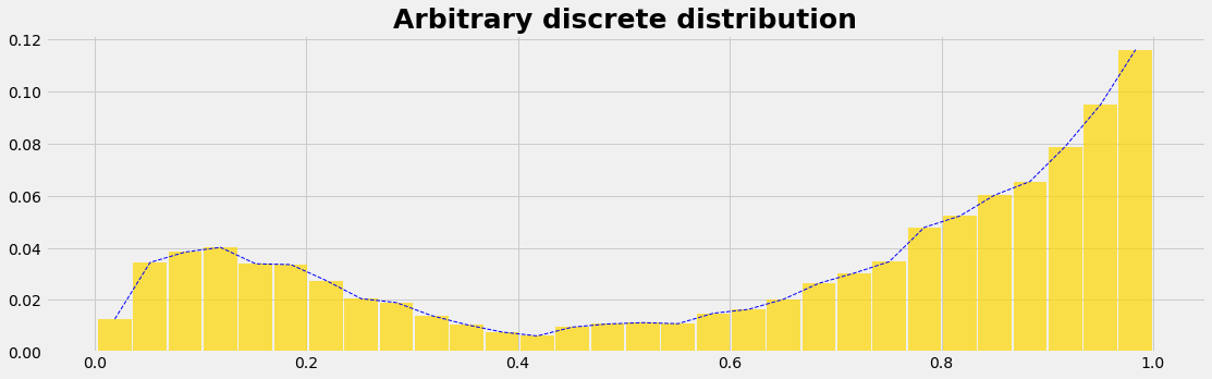
Let's assume we have a dataset we wish to use as a sampling engine. We'll assume the data:
- is Empirical
- is Discrete (given by data points)
- has an unknown function defining the distribution
If we want a random number generator that returns data with the same distribution of our empirical distribution we can do so in 3 steps:
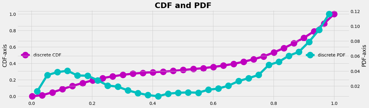
- Define a cumulative density function (CDF) for our empirical distribution (the cumulative sum from the PDF, ranging from [0,1] on the y-axis)
- Create a uniform random generator that gives data in the interval [0,1]
- Identify which element of the CDF the random number fits best and count the 'hit' (which is the x-axis transformation)
References
How to randomly sample your empirical arbitrary distribution
Forecasting with Geospacial Data
Geo-statistics is a subfield of statistics focused on spatial or spatiotemporal datasets, AKA data with location or longitudinal data with location.
In the following case, we have a large set of longitudinal data with location and we want to make guesses about the future in those locations. Not to be confused with kriging which is a gaussian process of estimating a variable at an unobserved location, based on the estimates of nearby or similar locations.
Fun fact: Many of the techniques we use today originated from mining engineers who desired to know what minerals might lay beyond a surface given a sample.
The following notes aim to provide the fundamentals of creating a network of connected spaces, and forecasting techniques for spatial network data.
Networks
A network is a discrete set of items (referred to as nodes) with some connection between them (referred to as edges). Typically, a graph network is represented mathematically as G = (N, E); with a set of N nodes and E edges.
Time Series
A parametric model can be used to describe a relationship between independent and dependent variables. It's not unusual for a time series to exhibit a trend, such as seasonality.
Think of a time series as a series of components:
- A trend-cycle component
- A seasonal component
- A remainder component
Advanced Machine Learning
Recall that in an ordinary multiple linear regression, we have a set of p predictor variables measuring some response variable (Y) to fit a model like:
$$ Y = \beta_0 + \beta_1 X_1 ... \beta_p X_p + \epsilon $$
Where beta represents the average effect of a unit increase in the predictor Xn (the nth predictor variable) and epsilon is the error term. The value for these beta coefficients is chosen using the least square method, which minimizes the sum of squared residuals (RSS), or the squared difference in observed minus expected outcome value.
$$ RSS = \Sigma (y_i - \hat y_i)^2 $$
Least Absolute Shrinkage and Selection Operator (LASSO)
When variables are highly correlated then coefficient estimates can have large variances leading to poor predictive accuracy.
Lasso regression is a regularization technique for linear regression models. Regularization is a statistical method to reduce errors caused by overfitting on training data. Instead of trying to minimize RSS, Lasso uses the equation:
Total Cost = Measure of Fit [RSS] + Measure of magnitude of coefficients
$$ Cost = RSS + \lambda \Sigma | \beta_n | ; \lambda \ge 0 $$
Lambda is the 'tuning' parameter, or shrinkage penalty, and measures the balance of fit and sparsity. When this term is 0 the parameter has no effect, and as it approaches infinity the shrinkage penalty becomes more influential.
- Start with full model (all possible features)
- "Shrink" some coefficients to 0 (exactly)
- Non-zero coefficients indicate "selected" features
The idea is to have as little bias as possible so the variance can be reduced, leading to a smaller mean squared error (MSE).
Note: This is very similar to ridge regression, except in ridge the coefficients are minimized toward 0 but must always be > 0
Lasso tends to perform better when only a small number of predictor variables are significant, and ridge when all coefficients have roughly equal importance. To determine which model is better use k-fold cross validation.
Process
- Calculate correlation matrix and variance inflation factor values (VIF) for all predictor variables
- Fit the lasso regression model and choose a value for lambda
- Compare to a another regression model by way of k-fold cross-validation
Code
# https://www.r-bloggers.com/2020/05/quick-tutorial-on-lasso-regression-with-example/

library(glmnet)
# Loading the data
data(swiss)
x_vars <- model.matrix(Fertility~. , swiss)[,-1]
y_var <- swiss$Fertility
lambda_seq <- 10^seq(2, -2, by = -.1)
# Splitting the data into test and train
set.seed(86)
train = sample(1:nrow(x_vars), nrow(x_vars)/2)
x_test = (-train)
y_test = y_var[x_test]
cv_output <- cv.glmnet(x_vars[train,], y_var[train],
                       alpha = 1, lambda = lambda_seq,
                       nfolds = 5)
# identifying best lamda
best_lam <- cv_output$lambda.min
best_lam


# Output
# [1] 0.3981072


# Rebuilding the model with best lamda value identified
lasso_best <- glmnet(x_vars[train,], y_var[train], alpha = 1, lambda = best_lam)
pred <- predict(lasso_best, s = best_lam, newx = x_vars[x_test,])
# Combine predicted and actual values
final <- cbind(y_var[test], pred)
# Checking the first six obs
head(final)


# Output
#            Actual    Pred
#Courtelary   80.2 66.54744
#Delemont     83.1 76.92662
#Franches-Mnt 92.5 81.01839
#Moutier      85.8 72.23535
#Neuveville   76.9 61.02462
#Broye        83.8 79.25439


# R-squared
actual <- test$actual
preds <- test$predicted
rss <- sum((preds - actual) ^ 2)
tss <- sum((actual - mean(actual)) ^ 2)
rsq <- 1 - rss/tss
rsq


# Inspecting beta coefficients
coef(lasso_best)


# Output
#6 x 1 sparse Matrix of class "dgCMatrix"
#                         s0
#(Intercept)      66.5365304
#Agriculture      -0.0489183
#Examination       .
#Education        -0.9523625
#Catholic          0.1188127
#Infant.Mortality  0.4994369
XGBoost
XGBoost is a software library installed independently from whatever language is used to interact with it. Most popular languages have an interface, and there is a CLI version.
The library is focused on computational speed and model performance, and there are a number of advanced features. As the name suggests it uses a model optimization technique called gradient boosting, or gradient tree boosting. Let's quickly review.
Gradient Boosting
The original paper: Greedy Function Approximation: A Gradient Boosting Machine [PDF], 1999
The objective is to minimize the loss of the model by adding 'weak learners' ( usually a decision tree) using a gradient-descent like procedure. It is considered a stage-wide additive model, and was the landmark in the use of differentiable loss functions. The technique could be applied beyond binary classification problems to regression, multi-class classification models and more.
How it works:
1. A loss function to be optimized
This depends on the type of problem being solved. In the case of a regression one may used squared error (RSS), and a classification problem might have a logarithmic loss.
The benefit of gradient boosting is it does not need to derive a new boosting algorithm for each loss function; it is generic enough that any differentiable function can be used.
2. A decision tree to make predictions
Specifically regression trees that output real values for model outputs. This allows subsequent model outputs to be added together, and 'correct' the residuals.
Trees are constructed in a greedy manner, choosing best split points based on purity scores (e.g. Gini index) to minimize the lost. It is common to constrain the tree in specific ways, such as max nodes, layers, splits, or leaf nodes.
3. An additive model to add weak learners to minimize the loss function
A gradient descent procedure is used to minimize the loss when adding trees.
Traditionally, gradient descent is used to minimize a set of parameters. Error or loss is calculated and weights are updated to minimize that error.
Instead of parameters we have decision tree regression models. After calculating the loss in a given model, we must add the tree/model that reduces the loss (i.e. follow the gradient). This is done by parameterizing the tree then modifying the parameters of the tree to move in the right direction by reducing the residual loss. The output of the new tree is then added to the existing sequence of trees in an effort to correct the final output of the model.
A fixed number of trees are added or training stops once loss reaches an acceptable level or no longer improves based on the validation set.
Common Enhancements to Gradient Boosting
- Tree Constraints - As mentioned above, constraints on number of leaves, nodes, etc.
- Shrinkage/Weighted Updates - The predictions of each tree are added together sequentially and the contribution of each tree added can be weighted to 'slow down' the learning algorithm.
- Random sampling/Stochastic Gradient Boosting - Instead of using the full dataset, at each iteration a sub-sample of the training data is used (without replacement) to fit the base learner.
- Penalized learning/Regularized Gradient Boosting - The decision trees can be made more complex by adding regularization terms (often called weights) to smooth the final learnt weights to avoid over-fitting. By design this tends to select a simple and predictive model.
XGBoost Features
XGBoost supports all of the above common enhancements. In addition the software library can run distributed, parallel, out-of-core, and with cache optimization to make best use of hardware. Additionally, it can automatically handle missing data and provide continued training for new data.
Even with all these cool features XGBoost will only take numeric data as input. Code your character inputs to factors to create a matrix.
I'm going to include a list of hyperparameters below; These provide a simple interface for complicated tuning variables.
Full reference: https://xgboost.readthedocs.io/en/latest/parameter.html
| Parameter | Explanation |
|---|---|
| eta | default = 0.3 learning rate / shrinkage. Scales the contribution of each try by a factor of 0 < eta < 1 |
| gamma | default = 0 minimum loss reduction needed to make another partition in a given tree. larger the value, the more conservative the tree will be (as it will need to make a bigger reduction to split) So, conservative in the sense of willingness to split. |
| max_depth | default = 6 max depth of each tree… |
| subsample | 1 (ie, no subsampling) fraction of training samples to use in each “boosting iteration” |
| colsample_bytree | default = 1 (ie, no sampling) Fraction of columns to be used when constructing each tree. This is an idea used in RandomForests |
| min_child_weight | default = 1 This is the minimum number of instances that have to been in a node. It’s a regularization parameter So, if it’s set to 10, each leaf has to have at least 10 instances assigned to it. The higher the value, the more conservative the tree will be. |
Once you have your boosting model prepared run xgb.train()and xgboost()to train the boosting model. Both return a wrapper of class xgb.Booster, but xgb.train is an advanced interface which xboost is a simple wrapper for the former.
One of the parameters set in xgboost()is nrounds - the max number of boosting iterations (AKA how many decision trees get added). Setting this too low will result in a model which is too simple, and setting it too high leads to overfitting. The goal is to find the middle ground.
We should cross-validate to determine the correct numbe of rounds and other hyperparameters. XGBoost has a function to do this for us: xgb.cv()
Code
# https://www.r-bloggers.com/2020/10/an-r-pipeline-for-xgboost-part-i/
# https://www.kaggle.com/c/titanic/data
#
library(xgboost)
library(Matrix)
library(xgboost)
library(ggplot2)
library(ggthemes)
library(readr)
library(dplyr)
library(tidyr)
library(stringr)
theme_set(theme_economist())
set.seed(1234) # For reproducibility.

directoryWhichContainsTrainingData <-  "./xg_boost_data/train.csv"
directoryWhichContaintsTestData <- "./xg_boost_data//test.csv"

titanic_train <- read_csv(directoryWhichContainsTrainingData)
titanic_test <- read_csv(directoryWhichContaintsTestData)

titanic_train <- titanic_train %>%
  select(Survived,
         Pclass,
         Sex,
         Age,
         Embarked)

titanic_test <- titanic_test %>%
  select(Pclass,
         Sex,
         Age,
         Embarked)

str(titanic_train, give.attr = FALSE)
## tibble [891 x 5] (S3: tbl_df/tbl/data.frame)
##  $ Survived: num [1:891] 0 1 1 1 0 0 0 0 1 1 ...
##  $ Pclass  : num [1:891] 3 1 3 1 3 3 1 3 3 2 ...
##  $ Sex     : chr [1:891] "male" "female" "female" "female" ...
##  $ Age     : num [1:891] 22 38 26 35 35 NA 54 2 27 14 ...
##  $ Embarked: chr [1:891] "S" "C" "S" "S" ...

previous_na_action <- options('na.action') #store the current na.action
options(na.action='na.pass') #change the na.action

titanic_train$Sex <- as.factor(titanic_train$Sex)
titanic_train$Embarked <- as.factor(titanic_train$Embarked)

#create the sparse matrices
titanic_train_sparse <- sparse.model.matrix(Survived~., data = titanic_train)[,-1]
titanic_test_sparse <- sparse.model.matrix(~., data = titanic_test)[,-1]

options(na.action=previous_na_action$na.action) #reset the na.action

str(titanic_train_sparse)
## Formal class 'dgCMatrix' [package "Matrix"] with 6 slots
##   ..@ i       : int [1:3080] 0 1 2 3 4 5 6 7 8 9 ...
##   ..@ p       : int [1:6] 0 891 1468 2359 2436 3080
##   ..@ Dim     : int [1:2] 891 5
##   ..@ Dimnames:List of 2
##   .. ..$ : chr [1:891] "1" "2" "3" "4" ...
##   .. ..$ : chr [1:5] "Pclass" "Sexmale" "Age" "EmbarkedQ" ...
##   ..@ x       : num [1:3080] 3 1 3 1 3 3 1 3 3 2 ...
##   ..@ factors : list()

dim(titanic_train_sparse)
## [1] 891   5
head(titanic_train_sparse@Dimnames[[2]])
## [1] "Pclass"    "Sexmale"   "Age"       "EmbarkedQ" "EmbarkedS"

# booster = 'gbtree': Possible to also have linear boosters as your weak learners.
params_booster <- list(booster = 'gbtree', eta = 1, gamma = 0, max.depth = 2, subsample = 1, colsample_bytree = 1, min_child_weight = 1, objective = "binary:logistic")

# NB: keep in mind xgb.cv() is used to select the correct hyperparams.
# Here I'm only looking for a decent value for nrounds; We won't do full hyperparameter tuning.
# Once you have them, train using xgb.train() or xgboost() to get the final model.

bst.cv <- xgb.cv(data = titanic_train_sparse,
              label = titanic_train$Survived,
              params = params_booster,
              nrounds = 300,
              nfold = 5,
              print_every_n = 20,
              verbose = 2)

# Note, we can also implement early-stopping: early_stopping_rounds = 3, so that if there has been no improvement in test accuracy for a specified number of rounds, the algorithm stops.

res_df <- data.frame(TRAINING_ERROR = bst.cv$evaluation_log$train_error_mean,
                     VALIDATION_ERROR = bst.cv$evaluation_log$test_error_mean, # Don't confuse this with the test data set.
                     ITERATION = bst.cv$evaluation_log$iter) %>%
  mutate(MIN = VALIDATION_ERROR == min(VALIDATION_ERROR))

best_nrounds <- res_df %>%
  filter(MIN) %>%
  pull(ITERATION)

res_df_longer <- pivot_longer(data = res_df,
                              cols = c(TRAINING_ERROR, VALIDATION_ERROR),
                              names_to = "ERROR_TYPE",
                              values_to = "ERROR")

g <- ggplot(res_df_longer, aes(x = ITERATION)) +        # Look @ it overfit.
  geom_line(aes(y = ERROR, group = ERROR_TYPE, colour = ERROR_TYPE)) +
  geom_vline(xintercept = best_nrounds, colour = "green") +
  geom_label(aes(label = str_interp("${best_nrounds} iterations gives minimum validation error"), y = 0.2, x = best_nrounds, hjust = 0.1)) +
  labs(
    x = "nrounds",
    y = "Error",
    title = "Test & Train Errors",
    subtitle = str_interp("Note how the training error keeps decreasing after ${best_nrounds} iterations, but the validation error starts \ncreeping up. This is a sign of overfitting.")
  ) +
  scale_colour_discrete("Error Type: ")

g

bstSparse <- xgboost(data = titanic_train_sparse, label = titanic_train$Survived, nrounds = best_nrounds, params = params_booster)
## [1]  train-error:0.207632
## [2]  train-error:0.209877
## [3]  train-error:0.189675
## [4]  train-error:0.173962
## [5]  train-error:0.163861
## [6]  train-error:0.166105
## [7]  train-error:0.166105
## [8]  train-error:0.162739
## [9]  train-error:0.156004

titanic_test <- read_csv(directoryWhichContaintsTestData)

predictions <- predict(bstSparse, titanic_test_sparse)
titanic_test$Survived = predictions

titanic_test <- titanic_test %>% select(PassengerId, Survived)
titanic_test$Survived = as.numeric(titanic_test$Survived > 0.5)
Support Vector Machine (SVM)
SVMs, AKA vector networks, are supervised max-margin models for classification and regression analysis. The concept is very easy to understand; We use data labels to generate multiple separating regions (called hyperplanes) that separate the data points.
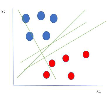
The goal is to maximize the margin, so that both groups of points are equidistant from the plane that divides them.
Hard margins are typically referred to as linear lines that can separate the data. Of course, this is a vast oversimplification. In reality, data is rarely linearly separable. Soft margins must be used to allow for weaker boundaries. This is where the support vector machine comes in.
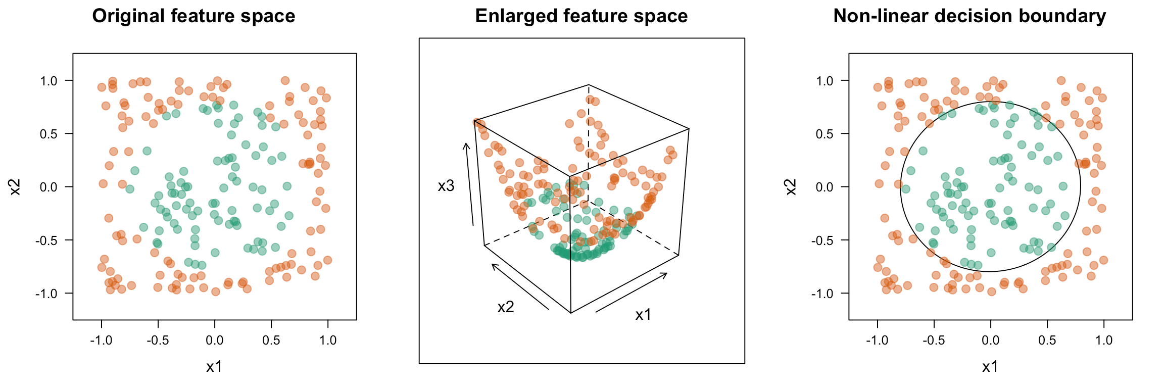
To adapt to nonlinear relationships SVM uses a kernel function. This is a mathematical function used to map input data into a high-dimensional feature space. Common kernel functions include:
- Linear AKA dot product - K(x, xi) = sum(x * xi)
- Polynomial - K(x,xi) = 1 + sum(x * xi)^d; When d=1 this is the same as linear regression. Manually setting d allows for curved lines in the input space
- Radial basis function - K(x,xi) = exp(-gamma * sum((x – xi^2)); Good for complex polygons
- & more
A key player in the kernel function are the support vectors, vectors which contain the data points closest to the hyperplane which divides the data.
This gives SVMs with proper training data a high predictive accuracy for classification tasks. However, one downside is there is no 'probability' in the sense of how effective a prediction is.
Code
dataset = read.csv('Social_Network_Ads.csv')
dataset = dataset[3:5]

# Encoding the target feature as factor
dataset$Purchased = factor(dataset$Purchased, levels = c(0, 1))

# Splitting the dataset into the Training set and Test set
install.packages('caTools')
library(caTools)

set.seed(123)
split = sample.split(dataset$Purchased, SplitRatio = 0.75)

training_set = subset(dataset, split == TRUE)
test_set = subset(dataset, split == FALSE)

dat = data.frame(x, y = as.factor(y)) # make output a factor
library(e1071) # contains svm function

classifier = svm(formula = Purchased ~ .,
                 data = training_set,
                 type = 'C-classification',
                 kernel = 'linear',
                 scale = TRUE) # do not scale
print(classifier)
plot(classifier, dat)


# Predicting the Test set results
y_pred = predict(classifier, newdata = test_set[-3])

# Making the Confusion Matrix
cm = table(test_set[, 3], y_pred)