# Module 9: Hypothesis Testing
The "effect" of a particular factor on some health outcome can be described as a parameter. Statistical hypothesis testing begins with a probability model assuming there is no effect or a **null hypothesis (H0)** and deciding whether there is sufficient evidence to reject the null hypothesis in favor of the **alternative hypothesis (H1).** Think of it like a legal trial; innocent until proven guilty.
One-sided Hypothesis: H0: θ = θ0 vs H1: θ > θ0 (or θ < θ0)
Two sided Hypothesis: H0: θ = θ0 vs H1: θ != θ0
We test H0 by finding an appropriate subset R ⊂ x, **the rejection region.** R is defined by R = {x : T(x) > c}; where T is a **test statistic** and c is a **critical value**.
- If X ∈ R -> reject null hypothesis
- If X !∈ R -> retain the null hypothesis
#### Errors
[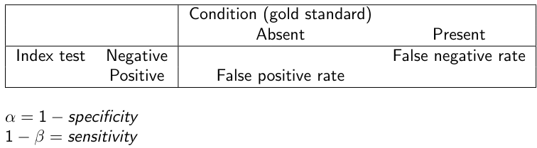](https://bookstack.mitchellhenschel.com/uploads/images/gallery/2022-08/image-1661437110788.png)
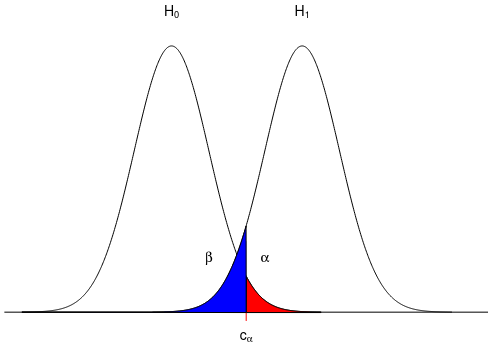
**Type I** **error** or **false positive** is rejecting H0 when it is true. α represents the probability of this error (typically set at .05)
**Type II error** or **false negative** is failing to reject the null when it is false. Probability represented by β.
[](https://bookstack.mitchellhenschel.com/uploads/images/gallery/2022-08/image-1661442140923.png)
#### Conducting and Interpreting the Test
1. Define null and alternative hypothesis
2. Set a desired α level. We choose a critical value such that: P(T(x) > c | θ = θ0) = α
3. Collect data
4. Calculate the observed test statistic value and compare to the critical value
5. Make decision
**P-value** is the smallest critical value at which the test leads to rejecting the null hypothesis. It is a probability, when assuming the null is true, of obtaining a test statistic at least as large as the one we observed.
- p < α -> reject null
- p > α -> retain null
Retaining the hypothesis does not mean the null is true, it is interpreted as a lack of evidence to accept the alternative.
[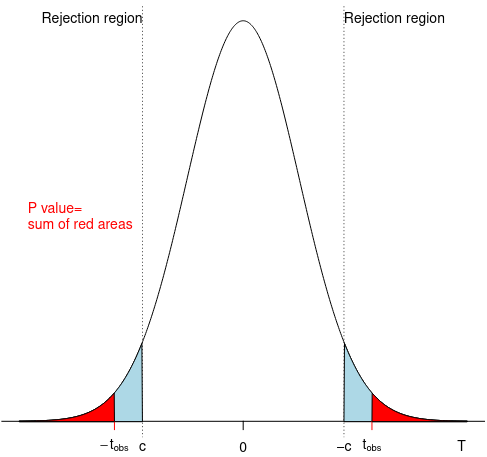](https://bookstack.mitchellhenschel.com/uploads/images/gallery/2022-08/image-1661438399131.png)
We expect the data to come from the center of the distribution, there is a lower probability of pulling data from tails. If our sample statistic occurs at the tail, then this may not be a representative distribution.
- The **power function** of a test with rejection region R is:
- Q(θ) = P(X ∈ R)
- The **size** of a test is defined as:
- S(θ) = sup(Q(θ))
- A test is said to have **level α** if its size is less than or equal α
- 1 - β is called the **power**, the probability of rejecting the null when the alternative of true
- The alternative corresponds to a range of value, thus power will depend on whatever alternative parameter value we choose to consider
- These quantities allow identifying the adequate critical value for the test
If variance is known we can use Z-scores to compare to our critical value:
[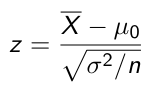](https://bookstack.mitchellhenschel.com/uploads/images/gallery/2022-08/image-1661440488199.png)
Otherwise use a t-distribution with n-1 degrees of freedom. A paired t-test is used when we are interested in the difference between two variables for the same subject when the null is that the mean difference is 0:
[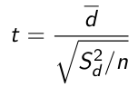](https://bookstack.mitchellhenschel.com/uploads/images/gallery/2022-08/image-1661440416881.png)
d represents the difference in sample mean differences and the denominator is the standard error.
Likewise, we can also use t and z scores to create tests for proportion:
[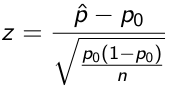](https://bookstack.mitchellhenschel.com/uploads/images/gallery/2022-08/image-1661440872693.png)
#### Relationship to Confidence Intervals
The null hypothesis can be tested against a two-sided alternative using a significance level α by assessing if the null parameter is contained in the 100(1 - α)% confidence interval for the parameter.
Also consider the comparison between two population means. If a confidence interval of the differences may not include zero while the CI of each population mean may overlap. So, overlapping intervals do not imply the samples have the same means.