# Module 6 & 7: Summary Statistics and Parameter Estimation
Since it is practically impossible to enroll the whole target population, we take a **sample -** a subgroup representative of the population. Since we're not examining the whole population, inferences will not be certain. **Probability** is the ideal tool to model and communicate uncertainty inherent with informing the population characteristic based on a sample. Inferences are categorized into two broad categories:
1. Estimation - Estimate the value of a parameter based on a sample
2. Hypothesis Testing - Comparing parameters fir two sub-populations using tests of significance
For smaller sample sizes (n < 30) we can use a t distribution.
### Parameter Estimation
In many statistical problems we make an assumption on the probability distribution from which the data are generated. The likelihood function is a concept that indicates how likely different parameters are to fit your distribution. Maximum likelihood is an approach based on selecting the parameter values that make the observed sample most likely.
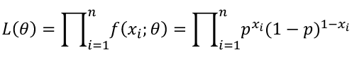
If Xi, ... Xn is a sample of independent observations from X~f(x; 𝜃), the likelihood function is defined as:
[](https://bookstack.mitchellhenschel.com/uploads/images/gallery/2022-08/image-1661264465927.png)
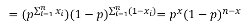
The product of each observation (marginals); As a joined distribution is the product of the marginals when the observations are independent (identically distributed). For binomial distributions, this can be further simplified:
[](https://bookstack.mitchellhenschel.com/uploads/images/gallery/2022-08/image-1661264635386.png)
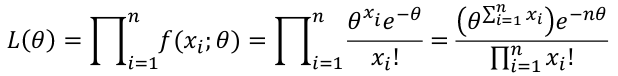
For a Poisson Likelihood with the mean -> p(X=x) = (𝜃xi\*e-𝜃)/x!; 𝜃 = mean
[](https://bookstack.mitchellhenschel.com/uploads/images/gallery/2022-08/image-1661265028248.png)
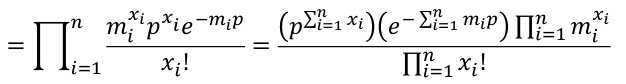
We could also express the Poisson likelihood function in terms of rates for each subject. So Xi ~ Poisson(mi\*p); where m is the number of trials and p is the probability of success, and assuming independence.
[](https://bookstack.mitchellhenschel.com/uploads/images/gallery/2022-08/image-1661266044271.png)
For a Normal Distribution likelihood can be expressed in terms of mean and variance:
[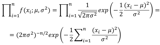](https://bookstack.mitchellhenschel.com/uploads/images/gallery/2022-08/image-1661266158661.png)
### MLE
The **Maximum Likelihood Estimate (MLE)** is the value of the parameter that maximizes the likelihood equation. Often we work with the log-likelihood because it will lead to the same maximize (since log is a strictly increasing function). To find this with calculus we can differentiate and set the derivative to 0.
#### Concepts
- An estimator T of a parameter 𝜃 us unbiased if E(T) = 𝜃
- The MLE 𝜃hat is not always unbiased. However, under general conditions the probability 𝜃 = 𝜃hat approaches 1 as the sample size n grows to infinity. (Consistency of MLE)
- The practicality of this is that MLE on average will approximate the true population value in large samples.
- When two estimators are unbiased one can compare them by variances. The best estimator would be the one with smaller variance -> more precise.
- To compare biased estimators we use mean squared error:
- MSE(T) = E(T - 𝜃)2 = (E(T) - 𝜃)2 + V(T) = bias(T)2 + V(T)
- Sometimes it is preferable to have a biased estimator with a low variance (bias-variance tradeoff)
In logistic regression we often take the log of the Odds Ratio.
[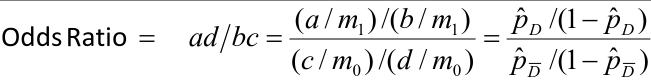](https://bookstack.mitchellhenschel.com/uploads/images/gallery/2022-08/image-1661268816285.png)
[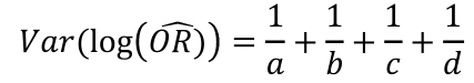](https://bookstack.mitchellhenschel.com/uploads/images/gallery/2022-08/image-1661268877129.png)
##### Binomial:
L(p) = px(1-p)n-x
l(p) = log(L(p)) = x\*log(p) + (n-x)\*log(1-p)
dl(p) / dp = x / p - (n-x) / (1 - p) = 0
(x\*(1 - p) - (n-x)\*(1 - p)) / (p\*(1 - p) = 0
x = np -> phat=x/n
Based on CLT, when n is large:
X ~ N(np, np(1-p)) and phat = X / n ~ N(p, p(1-p)/n)
##### Poisson:
For means:
[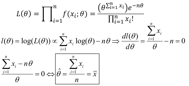](https://bookstack.mitchellhenschel.com/uploads/images/gallery/2022-08/image-1661266883776.png)
For Probabilities:
[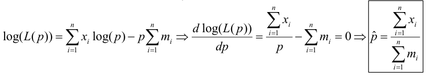](https://bookstack.mitchellhenschel.com/uploads/images/gallery/2022-08/image-1661266953089.png)
##### Normal Distributions:
[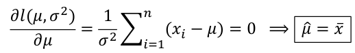](https://bookstack.mitchellhenschel.com/uploads/images/gallery/2022-08/image-1661267066196.png)
[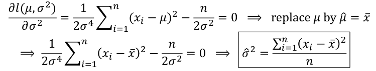](https://bookstack.mitchellhenschel.com/uploads/images/gallery/2022-08/image-1661267053502.png)
This looks very similar to our estimate of S2 or "Sample Variance" but has n in the denominator instead of (n-1), meaning this is biased at low sample sizes.
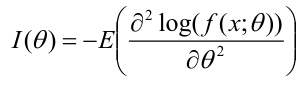
### Large Sample Approximation
Fisher Information Matrix can be used to forecast the precision in one observation:
[](https://bookstack.mitchellhenschel.com/uploads/images/gallery/2022-08/image-1661270408385.png)
This is a very important property that allows us to generate approximate distribution for MLE when the sample size is large.