# Module 4: Discrete Distributions
For any domain there are infinitely many distributions. The most common and famous distributions get a name; Binomial, Negative Binomial, Geometric, Hypergeometric, Poisson, etc. In this section we focus on Binomial and Poisson distributions.
The **Bernoulli** **Distribution** is a special member of the distribution family. It is the simplest example of a **Binomial distribution,** with only two domains (aka **dicothomous** distribution). A experiment which only has two domains is called a Bernoulli experiment. Ex. the number of students who get an A on a test, whether a person has a disease or not.
If we have two Bernoulli independent trials with equal probability of a positive result, **we refer to that probability as pi (not 3.14)**
X1 = { 1 if outcome +, 0 if outcome - } and X2 = { 1 if outcome +, 0 if outcome - }
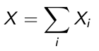
Then, X = X1 + X2
The variable X above is a random variable with domain of {0, 1, 2} as it is a result of the two trials. The distribution is an example of a Binomial (2, pi) distribution.
More generally, if Xi are n Bernoulli independent trials with probability of a positive result equals pi
[](https://bookstack.mitchellhenschel.com/uploads/images/gallery/2022-08/image-1660834298993.png)
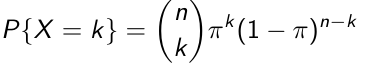
The domain of X a Binomial (n, pi) is {0, 1, 2... n}. When n=1 the binomial reduces to Bernoulli
For k in domain {0, 1, 2, ...n}:
[](https://bookstack.mitchellhenschel.com/uploads/images/gallery/2022-08/image-1660840678211.png)
This is only for = and not eqaullity
- Where (nk) = (n!) / (k! \* (n-k)!) Where n! = 1 \* 2 \* 3 \* ... n and 0! = 1
- Mean = μ = E \[X \] = nπ
- Variance = σ2 = Var \[X\] = nπ(1 − π)
Note that variance is a function of mean, Mean > Variance and for a fixed n the variance is maximum at pi = .5
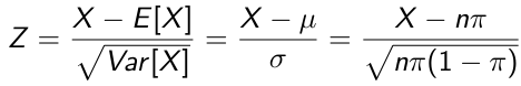
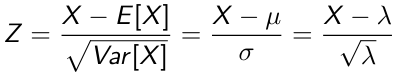
We can construct the standard Z score with:
[](https://bookstack.mitchellhenschel.com/uploads/images/gallery/2022-08/image-1660835389912.png)
We can use the Standard Normal Distribution to approximate a binomial distribution when n is large (say > 25), this is an example of the Central Limit Theorem. The **Central Limit Theorem** states if you take the sum of a large number of independent, identically distributed variables you can approximate the outcome under a normal distribution. This is the basis of inference in current applied statistics.
### Poisson Distribution
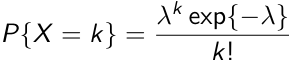
Named after the French mathematician who derived it; the first application was the description of the number of deaths as a result of horse kicking in the Prussian army. It can be used to model the number of events occurring within a given time interval. The probability density (mass) function is:
[](https://bookstack.mitchellhenschel.com/uploads/images/gallery/2022-08/image-1660837060834.png)
where λ is the mean of the distribution (mean number of events); λ determines the shape of the distribution. Other properties which make Poisson distribution popular:
- The mean and variance are both equal to λ
- The sum of independent Poisson variables is also (!) Poisson variable with mean equal to sum of the individual means
- Poisson distribution provides an approximation for the Binomial distribution
- The standard Z score:
[](https://bookstack.mitchellhenschel.com/uploads/images/gallery/2022-08/image-1660837263357.png)
If n is large and pi is small, the the Binomial distribution with parameters n and pi can be approximated by a Poisson distribution with mean parameter n\*(pi). From there probability calculations with Poisson reduce to probability calculations for a standard normal distribution.
When converting a discrete binomial distribution to a continuous distribution we must add correction for continuous conversions:
[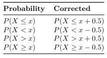](https://bookstack.mitchellhenschel.com/uploads/images/gallery/2022-08/image-1660847869791.png)
Think about it like this:
[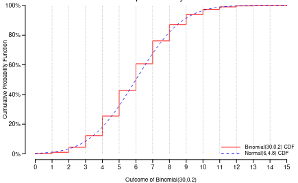](https://bookstack.mitchellhenschel.com/uploads/images/gallery/2022-08/image-1660870087072.png)
In a binomial distribution probability can only accumulate at discrete times {1, 2, 3,...} but since a normal distribution is continuous, you have to account for weather or not you want to include the point.
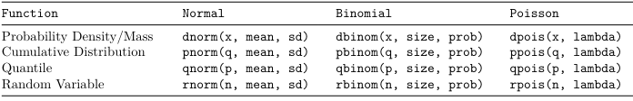
Useful R functions:
[](https://bookstack.mitchellhenschel.com/uploads/images/gallery/2022-08/image-1660852336215.png)
The general rule with functions in R:
- A single point (Probability Density Function) starts with d
- Cumulative Distribution starts with p
- Quantile starts with q
- Random variables start with r