Accelerated Statistical Training
BS800: Stats Boot Camp
A review of basic biostatistics jargon and methodology
- Module 1: Basics of Studies
- Module 2: Probability
- Module 3: Random Variables and Normal Distributions
- Module 4: Discrete Distributions
- Module 5: Multivariate Normal Distribution
- Module 6 & 7: Summary Statistics and Parameter Estimation
- Module 8: Interval Estimation
- Module 9: Hypothesis Testing
- Module 10: Confounding and MH Method
- Module 11: ANOVA - Analysis of Variance
- Module 12: Basic Genetics
- Module 13: Linear Regression
- Module 14: Topics in Linear Regression
Module 1: Basics of Studies
Questions when creating a study:
- Outcome of interest?
- Groups?
- Population?
- Type of Study?
Comparative studies are intended to show differences of an outcome between two or more groups.
Cross Sectional - Collected at one point in time
Longitudinal - multiple data sets collected at different points in time
Retrospective - Collecting "group data" on selected outcomes
Prospective - Collecting "outcome" on selected groups
Cohort studies gather data on groups of interest
| Study Design |
Pros |
Cons |
| Randomized trials |
Strength of evidence |
May be unethical |
| Cohort studies |
Relative risk |
Bias confounding |
| Case-Control studies |
Easy and inexpensive |
Bias confounding |
| Cross-sectional |
Simplest |
Weakest evidence |
Confounding occurs when a relationship between an exposure (risk factor) and a outcome (disease) is misrepresented because each of these variables is also related to a 3rd variable, the confounder. Ex. Ice cream sales and violent crimes both increase when it is hot outside.
Prevalence: The proportion of sampled individuals that possesses a condition of interest at a given time. Likelihood of being a case at a given point in time.
Incidence: The proportion of individuals that develop a condition of interest over a defined period of time. Risk of becoming a case over a period of time.
Interaction (Effect Modification) occurs when the magnitude of the effect of the primary exposure on an outcome (i.e., the association) differs depending on the level of a third variable.
Measures of Association
| Cases (Have Disease) |
Controls (No Disease) |
|
| Exposed |
a |
b |
| Unexposed |
c |
d |
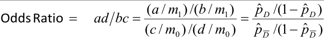
Odds Ratio (OR) = (a/c) / (b/d) = a*d / b*c = Odds that a Case was Exposed / Odds that a Control was Exposed
Relative Risk (RR) = (a / (a + b)) / (c / (c + d)) = Risk of Disease of Exposed / Risk of Disease Unexposed
If the OR is greater than 1 than the risk factor is associated with disease, less than 1 suggests its a protective factor and =1 suggests no association.
This is often used when searching for food-borne illnesses. They are quick and cheap, and can be used for uncommon disease. It falls short when finding rare exposures, and it can be difficult to find a representative control selection who can accurately recall if they were exposed.
The main measurement used in cohort studies is called the Relative Risk (RR), which is the risk of disease for those exposed to a risk factor over the risk of disease in the unexposed group.
RR > 1 is increased risk, RR < 1 is lower risk, RR = 1 is same risk
Mantel-Haenszel Method (mOR) is used to compare the odds ratio between two strata defined by counfounders. Ex. the rate of lung cancer in shipbuilders and non-shipbuilders, stratified on those who smoked. We would call this the OR adjusted by smoking.
Module 2: Probability
Probability is the study of uncertainty and randomness in the world. It measures chance.
Proportion is a summary statistic. Proportion measures size (i.e. how many patients have optional blood pressure).
- We show the probability of Event A as P(A)
- The compliment of an event, or chance of event not occurring is AC
- P(A) + P(AC) = 1
- Two events are mutually exclusive (or "disjoint") if when one event occurs the other cannot
- Two events are independent if the probability of one has no impact on the occurrence of the other
- Events are independent if:
- P(A|B) = P(A)
- P(A|B) = P(A| not B)
- Odds ratio = 1 (binary outcome)
- Events are independent if:
- If two events are not independent they are said to be statistically associated
- Joint Probability = P(A & B) = P(A,B) = P(A ꓵ B)
- If A and B are independent events: P(A & B) = P(A) * P(B)
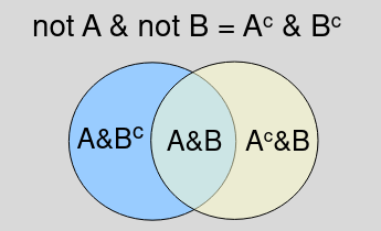
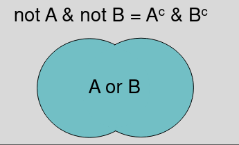
- P(A or B) = P(A U B)
- When A and B are non-mutually exclusive P(A or B) = P(A) + P(B) - P(A & B)
- When A and B are mutually exclusive events P(A or B) = P(A) + P(B) since P(A&B)=0
- Conditional probability is the chance of an event occurring given that another event occurred, written as P(A|B) = The probability of A given B.
- P(A|B) = P(A&B)/P(B)
- P(A|B) * P(B) = P(A & B)
Bayes' Theorem
Because P(A & B) = P(B & A),
P(A & B) = P(B & A) = P(B|A) × P(A)
=
P(A|B) × P(B) = P(B|A) × P(A)
P(B|A) = P(A|B) * P(B) / P(A)
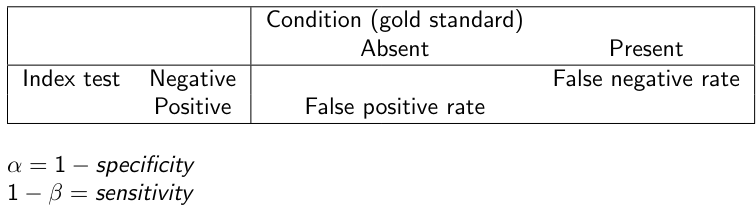
Sensitivity
Sensitivity of a screening test = Probability of positive test given the person has the disease. If X is the test result and Y represents if the person actually has the disease, this can be expressed as P(X = +| Y = +) = the probability of a disease given the test was positive.
Sensitivity = True Positive Fraction = P(Test+ | Disease)
Specificity = True Negative Fraction = P(Test - | No Disease)
False Positive = P(Test + | No Disease)
False negative = P(Test - | Disease)
Positive Predictive Value = P(Disease | Test +)
Negative Predictive Value = P(No Disease | Test -)
Odds Ratio
Odds ratio can be used to check independence, events are independent when OR=1.
OR = ( P(X = +| Y = +) / P(X = -| Y = +) ) / ( P(X = +| Y = -) / P(X = -| Y = -) )
= ( P(X = +| Y = +) * P(X = -| Y = -) ) / ( P(X = +| Y = -) * P(X = -| Y = +) )
Symmetry of Odds Ratio

Module 3: Random Variables and Normal Distributions
A variable is a measurement or characteristic on which individual observations are made. A random variable is a variable whose possible values are outcomes of a random phenomenon. A domain is a set of all possible values a variable can take.
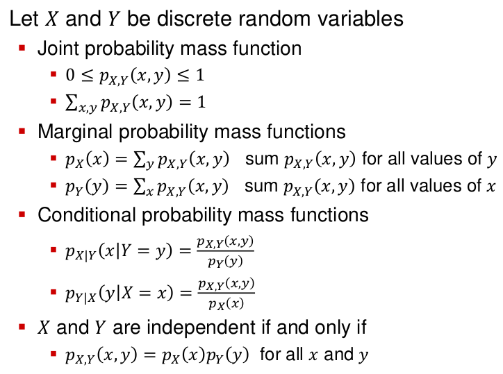
Discrete random variables is a finite set or countably infinite sequence.
px(xi) = P(X = xI) is called the Probability Mass Function (PMF).
- 0 <= px(xi) <= 1 as it is a probability,
- Sum of PMF for all values of X = 1.
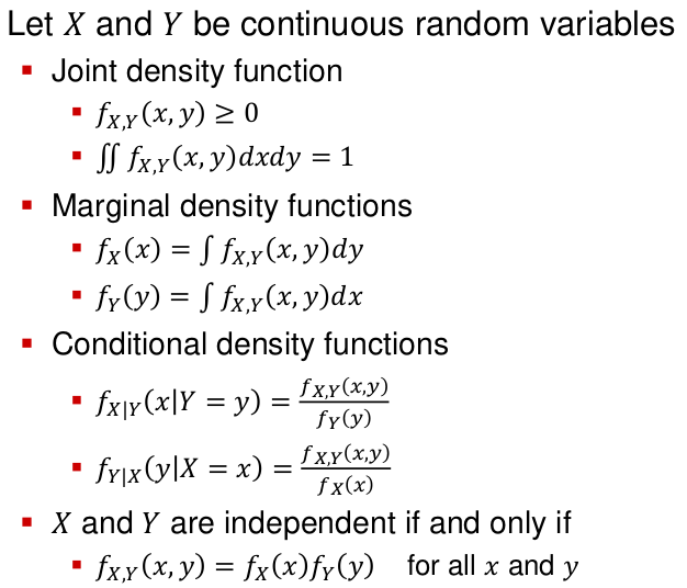
Continuous random variable can lie on a numerical scale, such as all real numbers between (0, +infinity). If we mapped the data to a histogram, we would see the curve begin to smooth as the number of data points approaches infinity.
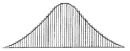
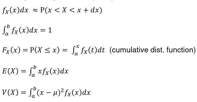
This density curve, fx(x), is called the Probability Density Function (PDF).
- fx(x) >= 0 but can be greater than 1
- The integral of fx(x) over the domain of X is 1
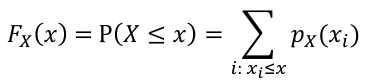
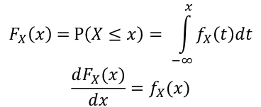
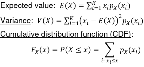
The Cumulative Distribution Function (CDF) is defined as Fx(X) = P(X <= x)
- Non-decreasing
- The limit toward -infinity is 0, toward +infinity is 1
- For discrete random variables:
- For continuous random variables:
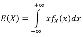
The Expected Value of a random variable is an average of the possible values weighted by their probabilities. Also called mean and denoted by μ.
- For discrete random variables
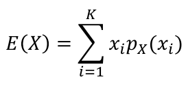
- For continuous random variables
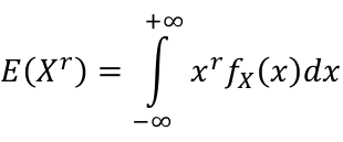
A generalization for the expected values is the rth moment of a random variables, R(Xr).
- For discrete random variables:
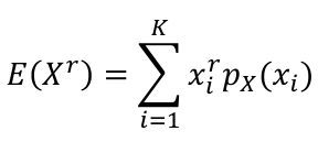
- For continuous random variables:
The first moment of a random variable is the expect value (mean). The rth moment of a random variable about the mean, also called the rth central moment, is defined as: E[(X - μ)r]
- The first central moment = 0
- The second central moment is the variance denoted as 𝜎2
The variance measures the spread around the mean of a random variable: Var(X) = E[(X - μ)2]
- Also equivelent to Var(X) = E(X2) - [E(X)]2
- The standard deviation is the square root of the variance
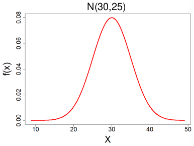
The normal distribution:
- is a continuous distribution
- can be expressed by a formula
- also called Gaussian distribution
- is a theoretical model for a population distribution that approximates the distribution of a number of measurement variables
- is appropriate for a number of measures, but not all. Only appropriate for some continuous measurements.
- is symmetric about the mean (i.e P(X > μ) = P(X < μ) = .5)
- is completely characterized mean and variance
The 68/95/99 rule:
- 68.25% of the data falls within 1 SD
- 95.45% of the data falls within 2 SD
- 99.74% of the data falls within 3SD
The standard normal random variable, referred to as Z, is in the scale of SD units from the mean.
Z has a μ=0 and SD = 1 we can standardize any normal distribution with:
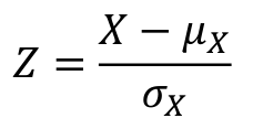
By converting to Z-scores we can easily compare the probability events in two different normal distribution.
The kth percentile is defined as the score that holds the k percent of the scores below it. Ex. 90th percentile is the score that has 90% of the scores below it. We can compute percentiles with: X = μ + Z𝜎
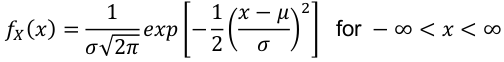
The probability density function for normal curves:
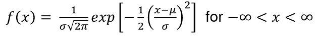
And in normal curves when mean is 0 and SD is 1 this can be simplified.
Relevant R Functions
qnorm(percentile, μ, 𝜎) computes percentiles for normal variables
dnorm(x, μ, 𝜎) will return the height of normal density function with a certain mean and SD at point x
pnorm(z, μ, 𝜎) will return the cumulative distribution function of a normal distribution with certain mean and SD
Module 4: Discrete Distributions
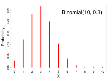
For any domain there are infinitely many distributions. The most common and famous distributions get a name; Binomial, Negative Binomial, Geometric, Hypergeometric, Poisson, etc. In this section we focus on Binomial and Poisson distributions.
The Bernoulli Distribution is a special member of the distribution family. It is the simplest example of a Binomial distribution, with only two domains (aka dicothomous distribution). A experiment which only has two domains is called a Bernoulli experiment. Ex. the number of students who get an A on a test, whether a person has a disease or not.
If we have two Bernoulli independent trials with equal probability of a positive result, we refer to that probability as pi (not 3.14)
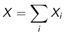
X1 = { 1 if outcome +, 0 if outcome - } and X2 = { 1 if outcome +, 0 if outcome - }
Then, X = X1 + X2
The variable X above is a random variable with domain of {0, 1, 2} as it is a result of the two trials. The distribution is an example of a Binomial (2, pi) distribution.
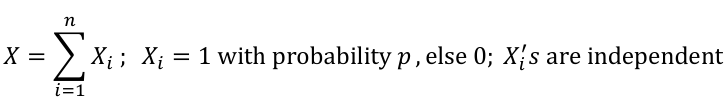
More generally, if Xi are n Bernoulli independent trials with probability of a positive result equals pi
The domain of X a Binomial (n, pi) is {0, 1, 2... n}. When n=1 the binomial reduces to Bernoulli
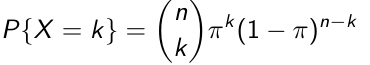
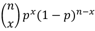
For k in domain {0, 1, 2, ...n}:
This is only for = and not eqaullity
- Where (nk) = (n!) / (k! * (n-k)!) Where n! = 1 * 2 * 3 * ... n and 0! = 1
- Mean = μ = E [X ] = nπ
- Variance = σ2 = Var [X] = nπ(1 − π)
Note that variance is a function of mean, Mean > Variance and for a fixed n the variance is maximum at pi = .5
We can construct the standard Z score with:
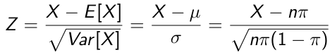
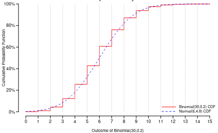
We can use the Standard Normal Distribution to approximate a binomial distribution when n is large (say > 25), this is an example of the Central Limit Theorem. The Central Limit Theorem states if you take the sum of a large number of independent, identically distributed variables you can approximate the outcome under a normal distribution. This is the basis of inference in current applied statistics.
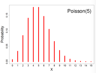
Poisson Distribution
Named after the French mathematician who derived it; the first application was the description of the number of deaths as a result of horse kicking in the Prussian army. It can be used to model the number of events occurring within a given time interval. The probability density (mass) function is:
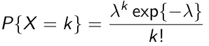
where λ is the mean of the distribution (mean number of events); λ determines the shape of the distribution. Other properties which make Poisson distribution popular:
- The mean and variance are both equal to λ
- The sum of independent Poisson variables is also (!) Poisson variable with mean equal to sum of the individual means
- Poisson distribution provides an approximation for the Binomial distribution
- The standard Z score:
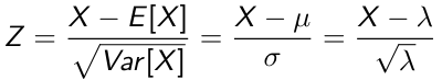
If n is large and pi is small, the the Binomial distribution with parameters n and pi can be approximated by a Poisson distribution with mean parameter n*(pi). From there probability calculations with Poisson reduce to probability calculations for a standard normal distribution.
When converting a discrete binomial distribution to a continuous distribution we must add correction for continuous conversions:
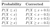
Think about it like this:
In a binomial distribution probability can only accumulate at discrete times {1, 2, 3,...} but since a normal distribution is continuous, you have to account for weather or not you want to include the point.
Useful R functions:
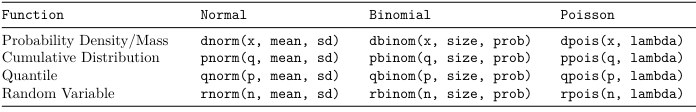
The general rule with functions in R:
- A single point (Probability Density Function) starts with d
- Cumulative Distribution starts with p
- Quantile starts with q
- Random variables start with r
Module 5: Multivariate Normal Distribution
A variable X follows a discrete probability distribution if the possible values of X are either:
- A finite set
- A countable infinite sequence
px(xi) = P(X=xi) is called the probability mass function (PMF)
- px(xi) >= 0 as it is a probability
- The sum of PMF for all values of X = 1
Recall that in a Discrete Probability Distribution :
In a Continuous Probability Distribution:
Because in a discrete set we are not concerned with the values in between our domain values.
Moment Generating Function
Moments are expected values of X, such as E(X), E(X2) = E(V), E(X3), etc. This, can also be calculated using the Moment Generating Function (MGF):
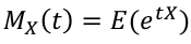
The rth moment of X, E(Xr) can be obtained by differentiating Mx(t) r times with respect to t and setting t=0
- Mx(0) = 1
- MIx(0) = E(X)
- MIIx(0) = E(X2) -> V(X) = MIIx(0) - (MIx(0))2
- In general, Mx(r)(0) = E(Xr)
In short, the nth moment is the nth derivative of MGF.
Uniqueness: if X and Y are two random variables and Mx(t) = My(t) when |t| < h for some positive number h, then X and Y have the same distribution
Note: MGF does not exist for all distributions (E(etx) may be infinity)
Important Distributions
Normal Distribution
X ~ N(μ, σ2) -infinity < μ < infinity , σ < 0
- PDF:
- E(X) = μ
- V(X) = σ2
- MGF:
Binomial Distribution
X ~ Binomial(n, p) 𝑝 ∈ [0, 1]
X = the number of successes in n trials when the probability of success in each trail is p.
We can think of X as the sum of n independent Bernoulli(p) random variables, with the same p for every Xi
- PMF:
- Expected value = E(X) = np
- Variance = V(X) = np(1-p)
- MGF = Mx(t) = (pet + (1-p))n
- Two discrete random variables are independent if: P(X = x & Y = y) = P(X = x)*P(Y=y)
Ex. A study which analyzed the prevalence of a disease in a population.
Poisson Distribution
X ~ Poisson(λ) λ > 0
X = The number of occurrences of an event of interest.
- PMF:
- Expected Values = E(X) = λ
- Variance = V(X) = λ
- MGF = Mx(t) = eλ(e^t - 1)
Poisson as an approximation of the Binomial Distribution
- If X ~ Binomial(n, p) and n -> infinity, p-> 0 such that np is a constant => X ~ Poisson(np)
- This assumes each event is independent
- Often used analyzing rare diseases
Ex. Analyzing lung cancer in 1000 smokers and non-smokers. This is binomial but can be estimated as a Poisson distribution.
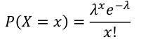
Geometric Distribution
X ~ Geometric(p) 𝑝 ∈ (0, 1]
If Y1, Y2, Y3 ... are a sequence of independent Bernoulli(p) random variables then the number of failures before the first success, X, follows a Geometric distribution.
- PMF = P(X = x) = p(1-p)x
- Expected value = E(X) = (1-p)/p
- Variance = V(X) = (1-p)/p2
- MGF = Mx(t) = p / (1 - (1 - p)et)
Ex. We want to know the number of times to flip a coin before it lands on heads.
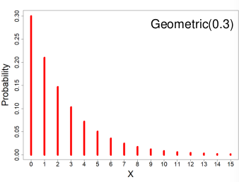
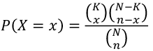
Hyper-Geometric Distribution
X ~ Hypergeometric(N, K, n)
Suppose a finite population of size N contains two mutually exclusive events: K success events and N-K failure events. If n events are randomly chosen without replacement X is the number of success events chosen.
- PMF:
- Expected value = E(X) = nk / N
- Variance = V(X) = ((nK) / N) * ((N-K) / N) * ((N - n) / (N - 1))
Ex. A bag has 7 red beads and 13 white beads. If 5 are drawn without replacement what is the probability exactly 4 are red?
Uniform Distribution
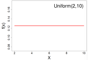
All outcomes are equally likely, they can be discrete or continuous.
X ~ Uniform(a, b) a < b
- PDF:
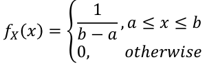
- E(X) = (a + b)/2
- V(X) = (b - a)2 / 12
- CDF = F(X) = (x - a) / (b -a), a<=x<=b
- MGF:
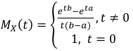
We use this distribution we use when we have no idea how the data is distributed.
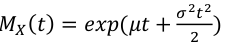
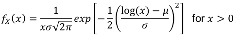
Log-Normal Distribution
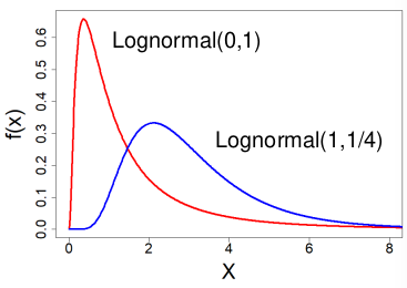
X ~ Lognormal(μ , σ2) -infinity < μ < infinity, σ > 0
- PDF:
- E(X) = exp(μ + σ2/2)
- Median = eμ
- V(X) = μ2 * (eσ^2-1)
- log(X) ~ N(μ, σ2) - the log is normal
- These distributions are often skewed to the right
Ex. Amount of rainfall, production of milk by cows, or stock market fluctuation often follow logarithmic functions.
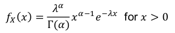
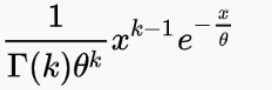
Gamma Distribution
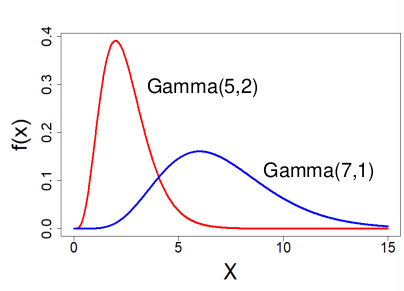
X ~ Gamma(α, λ) α > 0 , λ > 0
Used to predict the wait time until the first of event of something.
- PDF
Alternate paramterization with α > 0, 𝜃 = 1 / λ > 0 is used by R:
- E(X) = α / λ
- V(X) = α / λ2
- MGF:
Ex. Used to model time to failure or time to death.
Exponential Distribution
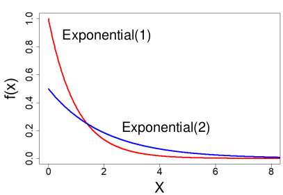
A special subset of the Gamma Distribution (α = 1)
X ~ Exponential(λ) λ > 0
- PDF = fx(x) = λ e-λ x for x > 0
- E(X) = 1 / λ
- V(X) = 1 / λ 2
- CDF = Fx(x) = 1 - e-λ x
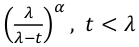
- MGF = Mx(t) = λ / (λ - t), t < λ
Ex. The time between geyser eruptions.
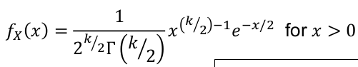
Chi-Square Distribution
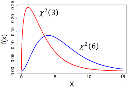
Special case of the Gamma Distribution (α = k/2, λ = 1/2)
X ~ X2(k) k is a positive integer (degrees of freedom, "df")
- PDF:
- E(X) = k
- V(X) = 2k
- MGF = (1 - 2t)-k / 2, t < 1/2
If you took a sample of Z scores and squared them you would have a chi-squared distribution with k = 1. Meaning, if Z1, Z2... Zm are independent standard normal random variables then:
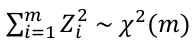
Very few real world distributions follow a chi-sqaure distribution, it is mainly used in hypothisis testing.
Bivariate Normal Distribution
A bivariate normal distribution is made up of two independent random variables. The two variables are both normally distributed, and have a normal distribution when added together.
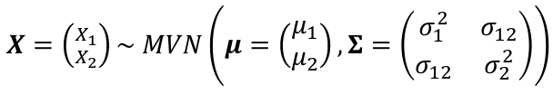
σ12 = Cov(X1, X2)
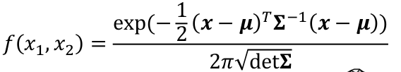
PDF:
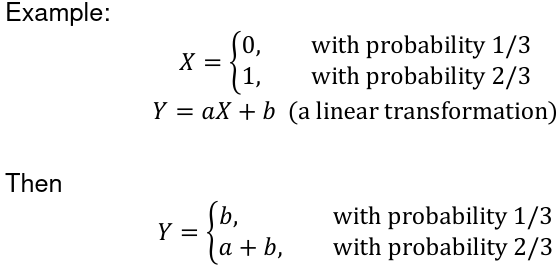
Function of a Discrete Random Variable
Suppose X is a discrete random variable and Y is a function of X. Y = g(X)
The Y is also a random variable: P(Y = y) = P(g(X) = y)
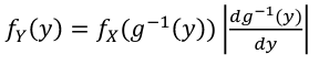
Function of a Continuous Random Variable
Using the same equation as above but assuming the variables are coninuous random variables:
The PDF = 
The CDF = 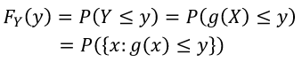
If g is one-to-one (strictly increasing or decreasing) then g has an inverse g-1, in the above case:
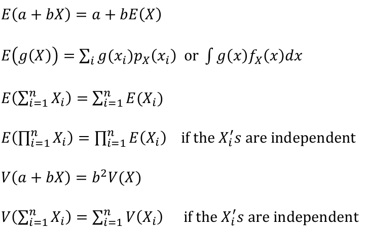
Properties of Expectation and Variance
Discrete Multivariate Distributions
Continuous Multivariate Distributions
Covariance and Correlation
Correlation is defined as an indication as to how strong the relationship between the two variables is:
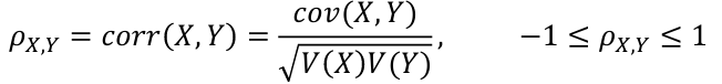
A positive correlation has σ > 0 and negative correlation has σ < 0
Covariance provides information about how the variables vary together:
cov(X, Y) = R[(X - E(X))(Y - E(Y))]
This is also equivalent to:
cov(X, Y) = E(XY) - E(X)*E(Y)
Thus if X and Y are independent:
cov(X, Y) = corr(X, Y) = 0
However cov(X, Y) = 0 does not imply indepence unless they are jointly normally distributed.
Conditional Expectation of X given Y = y, denoted E(X | Y = y):
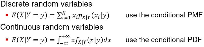
Conditional variance can be defined similarly (use the conditional PMF or PDF)
Module 6 & 7: Summary Statistics and Parameter Estimation
Since it is practically impossible to enroll the whole target population, we take a sample - a subgroup representative of the population. Since we're not examining the whole population, inferences will not be certain. Probability is the ideal tool to model and communicate uncertainty inherent with informing the population characteristic based on a sample. Inferences are categorized into two broad categories:
- Estimation - Estimate the value of a parameter based on a sample
- Hypothesis Testing - Comparing parameters fir two sub-populations using tests of significance
For smaller sample sizes (n < 30) we can use a t distribution.
Parameter Estimation
In many statistical problems we make an assumption on the probability distribution from which the data are generated. The likelihood function is a concept that indicates how likely different parameters are to fit your distribution. Maximum likelihood is an approach based on selecting the parameter values that make the observed sample most likely.
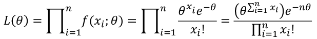
If Xi, ... Xn is a sample of independent observations from X~f(x; 𝜃), the likelihood function is defined as:
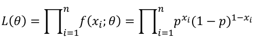
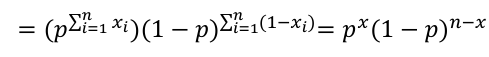
The product of each observation (marginals); As a joined distribution is the product of the marginals when the observations are independent (identically distributed). For binomial distributions, this can be further simplified:
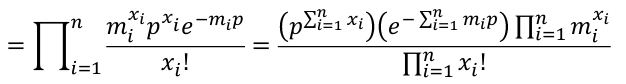
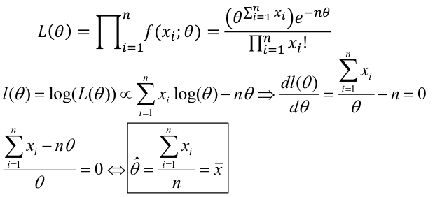
For a Poisson Likelihood with the mean -> p(X=x) = (𝜃xi*e-𝜃)/x!; 𝜃 = mean
We could also express the Poisson likelihood function in terms of rates for each subject. So Xi ~ Poisson(mi*p); where m is the number of trials and p is the probability of success, and assuming independence.
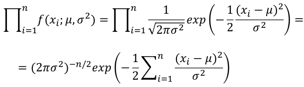
For a Normal Distribution likelihood can be expressed in terms of mean and variance:
MLE
The Maximum Likelihood Estimate (MLE) is the value of the parameter that maximizes the likelihood equation. Often we work with the log-likelihood because it will lead to the same maximize (since log is a strictly increasing function). To find this with calculus we can differentiate and set the derivative to 0.
Concepts
- An estimator T of a parameter 𝜃 us unbiased if E(T) = 𝜃
- The MLE 𝜃hat is not always unbiased. However, under general conditions the probability 𝜃 = 𝜃hat approaches 1 as the sample size n grows to infinity. (Consistency of MLE)
- The practicality of this is that MLE on average will approximate the true population value in large samples.
- When two estimators are unbiased one can compare them by variances. The best estimator would be the one with smaller variance -> more precise.
- To compare biased estimators we use mean squared error:
- MSE(T) = E(T - 𝜃)2 = (E(T) - 𝜃)2 + V(T) = bias(T)2 + V(T)
- MSE(T) = E(T - 𝜃)2 = (E(T) - 𝜃)2 + V(T) = bias(T)2 + V(T)
- Sometimes it is preferable to have a biased estimator with a low variance (bias-variance tradeoff)
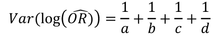
In logistic regression we often take the log of the Odds Ratio.
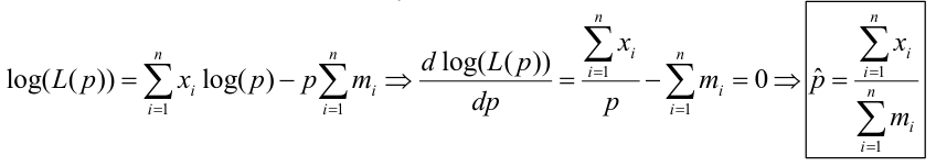
Binomial:
L(p) = px(1-p)n-x
l(p) = log(L(p)) = x*log(p) + (n-x)*log(1-p)
dl(p) / dp = x / p - (n-x) / (1 - p) = 0
(x*(1 - p) - (n-x)*(1 - p)) / (p*(1 - p) = 0
x = np -> phat=x/n
Based on CLT, when n is large:
X ~ N(np, np(1-p)) and phat = X / n ~ N(p, p(1-p)/n)
Poisson:
For means:
For Probabilities:
Normal Distributions:
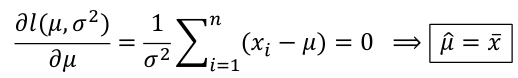
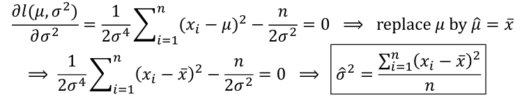
This looks very similar to our estimate of S2 or "Sample Variance" but has n in the denominator instead of (n-1), meaning this is biased at low sample sizes.
Large Sample Approximation
Fisher Information Matrix can be used to forecast the precision in one observation:
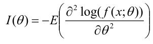
This is a very important property that allows us to generate approximate distribution for MLE when the sample size is large.
Module 8: Interval Estimation
- θ is fixed while θhat_n is a random variable which provides the single best value to estimate θ
- θhat is unbiased when bias = E(θhat_n) - θ = 0
- θhat is consistent when θhat_n -> θ
- Mean squared error MSE = E(θhat_n - θ)2 = bias(θhat_n) + V(θhat_n)
- If bias -> and se -> as n -> infinity then θhat_n is consistent
- Probability is stronger than samples, probability standard error eventually converges to 0 as n approaches infinity but samples converge to a normal distribution which is not necessarily the same as the population distribution.
- We the estimator variability (se) to provide an interval of parameter values that are "supported" by the sample.
A 1 - α confidence interval for a parameter θ is an interval Cn = (a; b) where a = a(X1, ...Xn) and b = b(X1, ...Xn) are functions of the data such that: P(θ ∈ Cn) >= 1 - α ; Where θ is the actual population mean. Cn is random and θ is fixed.
The confidence interval (a; b) capture the true mean with confidence 1 - α. We commonly use 95% confidence intervals which corresponds to α = .05. This does NOT mean there is 1- α chance/probability the parameter falls in the interval. The correct interpretation: If we repeatedly take samples of size n from a fixed and stable population and build a 95% confidence intervals, 95% of these intervals would contain the true unknown parameter.
CI For Mean of a Normal Distribution
If σ2 is known: Xbar +/- Zα/2*αx
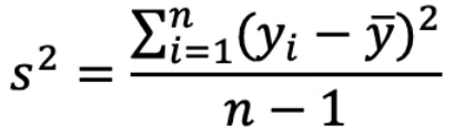
If σ2 is unknown: Xbar +/- t(α/2,n-1)*S/sqrt(n); Where S2 = 1/(n-1) * sum(xi-xbar)2
Using S in place of SD causes more uncertainty, thus increasing the size of the CI.
We can similarly find the confidence interval of a proportion in a similar manner:
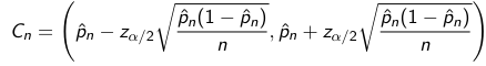
Chi-Square DIstribution
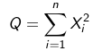
The above represents the chi-squared distribution with n degrees of freedom. E(Q) = n and V(Q) = 2n.
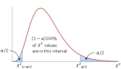
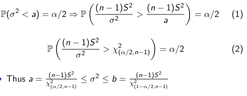
The distribution of X2n-1 is not symmetrical, so instead of centering our CI (a,b) on the mean, we look for symmetry so that the bounds P(θ < a) = α/2 and P(θ > b) = α/2.
We derive the variance of a distribution through Fisher's theorem (not shown). The CI comes out to:
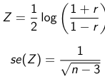
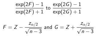
Pearson's product Moment Correlation Coefficient is between -1 and 1 and represents the correlation between 2 variables.
Although rarely used, you could find a confidence interval for this value.
Module 9: Hypothesis Testing
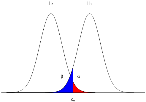
The "effect" of a particular factor on some health outcome can be described as a parameter. Statistical hypothesis testing begins with a probability model assuming there is no effect or a null hypothesis (H0) and deciding whether there is sufficient evidence to reject the null hypothesis in favor of the alternative hypothesis (H1). Think of it like a legal trial; innocent until proven guilty.
One-sided Hypothesis: H0: θ = θ0 vs H1: θ > θ0 (or θ < θ0)
Two sided Hypothesis: H0: θ = θ0 vs H1: θ != θ0
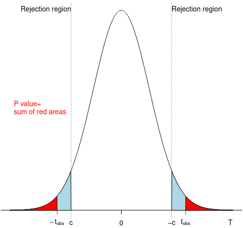
We test H0 by finding an appropriate subset R ⊂ x, the rejection region. R is defined by R = {x : T(x) > c}; where T is a test statistic and c is a critical value.
- If X ∈ R -> reject null hypothesis
- If X !∈ R -> retain the null hypothesis
Errors
Type I error or false positive is rejecting H0 when it is true. α represents the probability of this error (typically set at .05)
Type II error or false negative is failing to reject the null when it is false. Probability represented by β.
Conducting and Interpreting the Test
- Define null and alternative hypothesis
- Set a desired α level. We choose a critical value such that: P(T(x) > c | θ = θ0) = α
- Collect data
- Calculate the observed test statistic value and compare to the critical value
- Make decision
P-value is the smallest critical value at which the test leads to rejecting the null hypothesis. It is a probability, when assuming the null is true, of obtaining a test statistic at least as large as the one we observed.
- p < α -> reject null
- p > α -> retain null
Retaining the hypothesis does not mean the null is true, it is interpreted as a lack of evidence to accept the alternative.
We expect the data to come from the center of the distribution, there is a lower probability of pulling data from tails. If our sample statistic occurs at the tail, then this may not be a representative distribution.
- The power function of a test with rejection region R is:
- Q(θ) = P(X ∈ R)
- The size of a test is defined as:
- S(θ) = sup(Q(θ))
- A test is said to have level α if its size is less than or equal α
- 1 - β is called the power, the probability of rejecting the null when the alternative of true
- The alternative corresponds to a range of value, thus power will depend on whatever alternative parameter value we choose to consider
- These quantities allow identifying the adequate critical value for the test
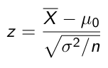
If variance is known we can use Z-scores to compare to our critical value:
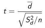
Otherwise use a t-distribution with n-1 degrees of freedom. A paired t-test is used when we are interested in the difference between two variables for the same subject when the null is that the mean difference is 0:

d represents the difference in sample mean differences and the denominator is the standard error.
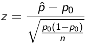
Likewise, we can also use t and z scores to create tests for proportion:
Relationship to Confidence Intervals
The null hypothesis can be tested against a two-sided alternative using a significance level α by assessing if the null parameter is contained in the 100(1 - α)% confidence interval for the parameter.
Also consider the comparison between two population means. If a confidence interval of the differences may not include zero while the CI of each population mean may overlap. So, overlapping intervals do not imply the samples have the same means.
Module 10: Confounding and MH Method
With categorical data, we are classifying data instead of measuring it. As a review:
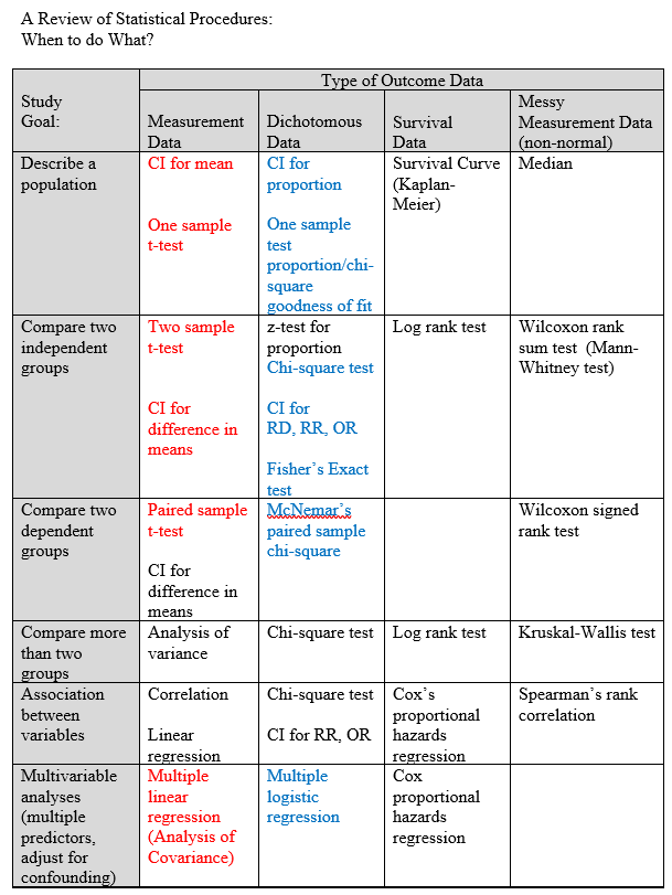
Notice we never use a z test, a t test is almost always more appropriate even for large samples. Likewise, for dichotomous outcomes could use a z-test but a chi-square test is usually used in practice. Chi-square reflects categorical outcomes.
chi-square = sum((obs-exp)2 / exp), df=n-1; where n is the number of random variables or categories.
Mantel-Hansel Method
Cochran-Mantel-Haenszel method is a technique that generates an estimate of an association between an exposure and an outcome after adjusting for or taking into account confounding. We stratify the data into two or more levels of the confounding factor (as we did in the example above). In essence, we create a series of two-by-two tables showing the association between the risk factor and outcome at two or more levels of the confounding factor, and we then compute a weighted average of the risk ratios or odds ratios across the strata
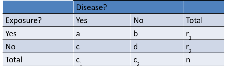
Given the above table, we have the below MH Equations:
For Cell(1,1) frequency has
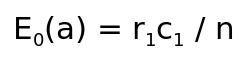
and
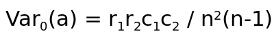
For a given table, and the MH test statistic is:
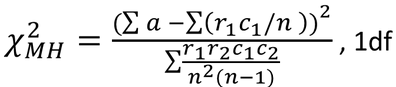
It follows a Chi-Square distribution with 1 degree of freedom.
We can also derive the following:
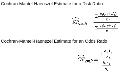
Though, in practice we just have the computer solve for MH estimates.
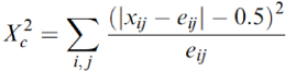
Continuity Corrections
Chi-Squared distributions are continuous whereas some variables are categorical, therefore we must correct by adding or subtracting .5. The "corrected" result is more accurate. This is often used when there are small samples or 0's in some cells.
Fisher's Exact Test
When a single epected value is small (n<5) a continuity correction only helps so much. In such cases we use Fisher's Exact test. Prepare your 2x2 table with the cell containing the smallest number in the upper left corner. Then identify all possible tables with that cell the same as or more extreme than observed and sum the probabilities. This gives the probability of that specific table.
Pr(a,b,c,d) = [(a+b)!(c+d)!(a+c)!(b+d)!] / N!a!b!c!d!
Again, this is usually performed by a computer. In R: fisher.test(Count)
Module 11: ANOVA - Analysis of Variance
ANOVA can be used to compare the means of several populations with continuous populations simultaneously. The population variance of the dependent variable must be equal in all groups.
Recall that
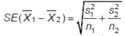
Which is the difference in two means over the standard error. When comparing multiple independent samples it is easier to use a pooled variance, but to do so the variances must be equal.
Equality of Variances
The equation for pool variance:
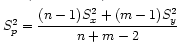
Assumption for pooled variance is that variances in the two groups are equal. We can test this with H0 = σ1=σ2 and use the F distribution which is indexed by the denominator df and the numerator df; choose the larger estimated variance to be numerator and the smaller estimated variance to be the denominator.
Test statistic:

If F is greater or smaller than critical values for a given significance level the null hypothesis is rejected and we can conclude there is evidence the two population variances are not equal.
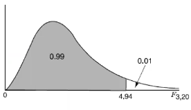
The F distribution is not symmetric, which makes it hard to look up critical values. It can be done in R: pf(F, df1, df2, lower=F)
The F test is not always appropriate as it is sensitive to departures from normality. Examine variability in the two groups by comparing sample variances using boxplots to help decide which standard error is appropriate. In the case where variances are unequal we use the same procedure but SE is estimated as:
Using the n-1 degrees of freedom from whichever sample is smaller as an approximate (SAS or R would figure out the exact value).
ANOVA
Terminology:
- Factor - category/grouping variable
- Level - individual group of the factor
- Balanced design - same number of individuals in each level
The general data configuration is we have k population groups each with nk observations, which can be the same or different.
Assumptions:
- Observations are independent
- Data are random samples from k independent populations
- Within each population the dependent variable is normally distributed
- The population variance of the dependent variable is equal in all groups.
H0: The k populations means are equal
Ha : The k populations means are not all equal or at least one is not equal
Recall that variance as a function of Y is:
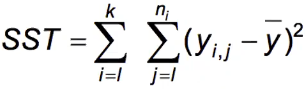
The numerator is the "Total variability" or the "Total sum of squares" (SST)
In ANOVA we split the SST into two components:
- Variability due to differences between the groups (SS Between Groups)
- Variability due to differences between individual y values within the groups (SS Within Group)
Which can also be expressed as:
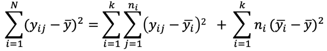
SS Total = SS Within Groups + SS Between Groups
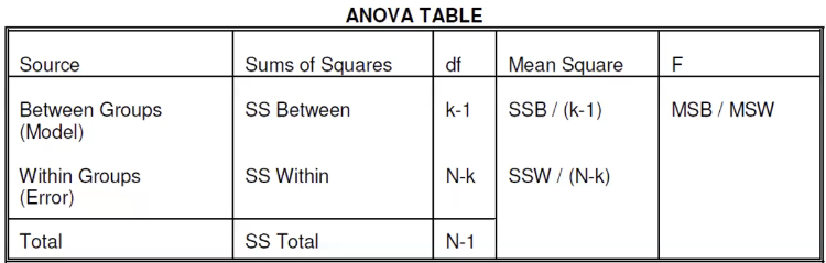
R2 is the proportion of variability explained by the difference between groups:
R2 = SS Between / SS Total
Adjustment Procedures
- Tukey's adjustment is appropriate when comparing pairs of means and is among the most powerful
- Provides exact P-values when groups are equal sizes
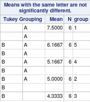
In the above Turkey procedure we observe group 1 and 3 are significantly different
- Scheffe's adjustment is appropriate for general contrasts
- Bonferroni's adjustment is appropriate for any situation but can be too conservative
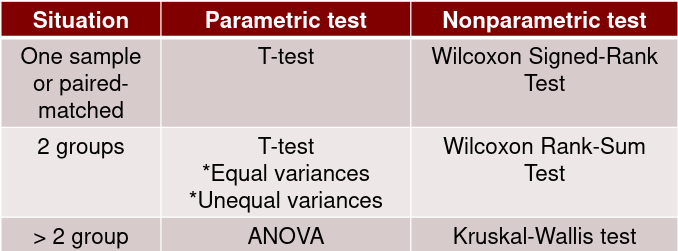
Parametric vs Non-parametric Tests
Tests are parametric because they make assumptions about the distribution of the data.
Non-parametric methods make fewer and more generic assumptions about the distribution of the data. These tests are generally more friendly toward non-normal distributions and small sample sizes.
Sign Test
Simplest non-parametric test. Analyze only the signs of the differences:
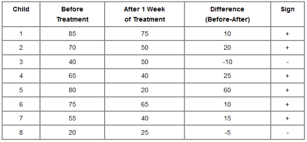
H0: The median difference is zero (half the signs are positive and half are negative)
Ha: The median difference is not zero
Wilcoxon Signed-Rank Test
Paired-sample t-test equivalent. Uses information on the relative magnitude of the paired differences as well as their signs.
Assumption:
- Independent observations
- Continuous or ordinal observations
- Symmetric distribution
H0: The median difference is zero
Ha: The median difference is not zero
1. Rank the magnitude of the differences (ignoring the signs)
2. Attach the signs to the ranks to form signed ranks
3. Calculate the test statistic, R, which is the sum of the positive ranks.
4. n≥20 → normal approximation
The values of the test statistic will range from 0 to N(N+1)/2, with a mean value of N(N+1)/4
Wilcoxon Rank-Sum Test
For two independent samples
Assumption:
- Independent observations
- Continuous or ordinal observations
- If using as a test of median, samples must have the same shape
H0: Distributions of populations from which the two groups are samples are the same.
Ha: Distributions of populations from which the two groups are samples are not the same.
1. Combine the two groups into one large sample and rank the observations from smallest to largest. Tied observations are assigned a average rank to all measurements with the same value.
2. Sum the ranks of each of the original groups.
3. The Wilcoxon sum rank test statistic (R) is the sum of the ranks in the group with the smallest sum
Kruskal-Wallis Test
A non-parametric analogue to one-way ANOVA. It's an extension of the Wilcoxon rank-sum test for more than two groups. Based on ranked data. The Kruskal Wallis test will tell you if there is a significant difference between groups. However, it won’t tell you which groups are different.
Assumption:
- Use when normality assumption is violated.
- Samples drawn from population are random
- Observations are independent
- The dependent variable is at least ordinal
- All groups have the same distribution shape
H0: The population medians are equal in all groups
Ha: At least one of the groups population median is different
Step 1: Rank data without respect to group (rank the data from 1 to N ignoring group membership).
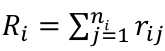
rij = rank of yij
Tie values obtain the rank of the average rank they would receive if not tied
Step 2: For each group i, compute
Step 3: Calculate h*
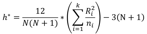
When H0 is true, h* has an approximate chi-square distribution with k-1 degrees of freedom
When we have tied values, need to make additional adjustments to h.
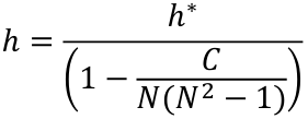
If g is the categories of tied values, the Lth category can be described as cL = m * (m2 - 1), where m is the number of ties values for the Lth category. The correction factor is C = c1 + c2 + ... + cg
Module 12: Basic Genetics
People are made of organs, organs are made of cells, cells are composed with genetic information. Genetics are important because we can earlier detect genetic diseases when a newborn has a genetic predisposition to disease; Ex. Cystic Fibrosis is a recessive gene. Complex traits are made up of more than one gene.
We can also use genetic information to create "custom drugs" in a practice called pharmacogenetics. Genetic factors account for 20% to 40% of inter-individual differences in metabolism and response. Genetic variants can alter the pharmacodynamics of a drug, potentially increasing efficacy or toxicity.
Somatic Cell Structure of Eukaryotes
All living things are made of cells. There are two types of cells:
- Somatic - differentiate to create organs required by an organism
- Germ (sex)
From a genetics POV the most important part of the cell is the nucleus, where the chromosomes are stored. Humans have 23 pairs of chromosomes, each set has 1 from the mother and 1 from the father. They are ordered from largest to smallest, (1 is largest, 22 is smallest). The 23rd is the sex chromosome, which is XX is females and XY in males.
DNA
Chromosomes are made up of Deoxyribonucleic acid (DNA) molecules. DNA molecule is packaged into chromosomes in a double helix ladder structure. The "rungs" of this ladder are bases or nulceotides. The two strands of the helix are complementary.
Nucleotides:
- Purines: Adenine and Guanine (A, G)
- Pyrimidines: Thymine and Cytosine (T, C)
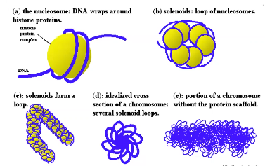
DNA Packaging
DNA molecules are packaged in a complex manner into chromosomes.
 c
cIn each cell there's nearly seven ft of DNA.
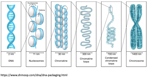
DNA is not tightly packed into chromosomes all the time, it only condenses when the cell is getting ready to divide.

Cytogenetic Location
Each human chromosome has a short arm ("p" for petite) and a long arm ("q" for queue), seperated by a centromere. The ends of the chromosome are called telomere. Each chromosome arm is divided into cytogenetic bands that can be seen using a microscope and special stains. At higher resolutions sub-bands are seen within bands.

These bands are numbered p1, p2, p3... q1, q2... etc. Counting from the centromere out toward the telomeres. This is the process geneticists use to address the location of a band or a range of bands of a gene.
Ex. 7q31.2 indicates it is on chromosome 7, q arm, region 3, band 1, and sub-band 2. The ends of chromosomes are labeled ptel and qtel; 7qtel refers to the end of the long arm on chromosome 7.
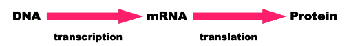
RNA
DNA codes for RNA which codes for protiens
- RNA is Ribonucleic acid
- Single strand
- Copies (transcribes) DNA to bring message to ribosomes for translation into proteins
- Uracil instead of thymine (U instead of T)
DNA "unzips" and allows RNA to transcribe it's molecules, then is transported to ribosomes in the cytoplasm. RNA is synthesized from 5' to 3'. This strand is called the template strand of DNA, and is complementary to the newly synthesized RNA while the coding strand of DNA has the same sequence as the new RNA. Either strand of the chromosome can take any role.
Proteins
Proteins are often referred to as the machinery of the cell as they are responsible for nearly every task in a cell. There are 20 "letters" in the protein alphabet, called amino acids.
The DNA alphabet (A,C,G, T) is transcribed into mRNA and then translated to proteins using codons. Codons consist of 3 DNA bases or letters; 43 = 64 combinations.
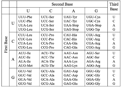
You'll notice some of these result in the same amino acids.
Gene Structure
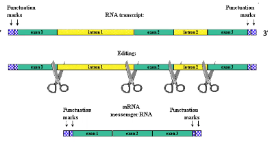
A gene, or a code for a specific protein sequence, does not lie in contiguous DNA - the RNA transcript is edited to create mRNA. The part that is removed is called the introns, and the parts kept are exons.
A gene is part of the DNA in the genome that is turned to RNA. They have several components:
- Promoter Region - Signals start of the gene. Often includes many A & T bases
- Exons - Translated from DNA to RNA then transcribed into proteins, expressed
- Introns - Cut out before protein transcription, unexpressed
- Splice site - junction of interon and exon, additional cutting my occur at these sites to produce different versions of proteins. Also called in between genes or intervening sequence (IVS)
Intron and Exon sizes vary between genes and thus can contain different number of base pairs.
Non-coding DNA (ncDNA)
Defined as all of the DNA sequences within a genome that are not found within protein-coding exons; Both inrons and IVS. Not represented within the amino acid sequence of expressed proteins. >98% of the human genomes is composed of ncDNA, and there are many different subtypes of ncDNA such as:
- Pseudogenes - regulatory DNA sequences, repetitive DNA sequences and sequences related to mobile genetic elements
- Sequences within genes:
- Genes for non-coding RNA (e.g. tRNA, rRNA)
- Untranslated components of protein-coding genes (introns, and 5' and 3' untranslated regions of mRNA)
Genetic Variability
There are genetic differences between humans. The different variations of a particular genetic location are called alleles. Since every chromosome is part of a pair each person has 2 alleles for every gene. The observed physical outcome of a gene is called the phenotype.
There are 3 billion base pairs in the human genetic sequence, taking up about 3GB of space on a computer. The DNA sequence across humans is 99.9% identical. That .1% results in differences across the genome.
Types of Genetic Variability
- Single base pair substitution - change in a single base pair.
- Sometimes called point mutation, single nucleotide polymorphism or "SNP"
- Polymorphism - DNA sequence variation that is common in the population (1% or higher). Alleles that occur with <1% frequency are called mutations
- Also called single nucleotide variant or "SNV", which also applies to mutations.
- Sometimes called point mutation, single nucleotide polymorphism or "SNP"
- Single Nucelotide Variant (SNV)
- Exonic
- Scilent/synonymous - it does not change amino acid due to degenerate code
- e.g. AAA -> AAG still codes for Lysine
- Nonsynonymous - changes animo acid sequence
- Missense -> changes a single amino acid
- Scilent/synonymous - it does not change amino acid due to degenerate code
- Non-Exonic - Intronic or intervening sequence
- Can be a single base change, insertion, or deletion
- Not part of the mRNA, so it will not alter the amino acid sequence
- Exonic
Sources of Genetic Variability
- Nucleotide repeats
- Can be caused by disease such as Huntington's Disease
- Copy Number Variants
- Gain and losses of large chunks of DNA sequence (10k - 5 million bases)
- Structural change in genome
- Found in exonic, intronic, and IVS
- ~.4% of genomes of unrelated people differ with respect to copy number
- Gain and losses of large chunks of DNA sequence (10k - 5 million bases)
Consequences of Genetic Polymorphism
- Change level of protein expression]
- Alter protein or make it non-functional
- Eliminate protein expression
- Create new protein
- Nothing
Representation of Genotypes
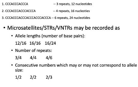
A person's genotype at a specific location in the genome consists of two alleles. There is not a standard way to record genotypes but some common conventions are concatenation, slashes and spaces:
11, 12, 22, 11 1/1,1/2,2/2,1/1 1 1, 1 2, 2 2, 1 1
For mutiallelic markers, markers with more than two alleles:
Module 13: Linear Regression
Correlation and regression attempt to describe the strength and direction of the association between two (or more) continuous variables.
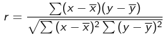
Pearson Correlation
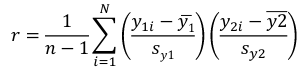
Recall r is an estimate of population correlation coefficient:
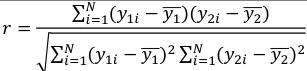
It is always between -1 and 1. With 0 indicating no positive or negative linear relationship between the variables.
A strong correlation does not imply causality.
It indicates the strength and direction of a linear relationship between two random variables. The square of r, r2 = R, measures how much information is shared between two variables; It is also called the coefficient of determination.
R2 can be explained as the proportion of the variability in y that can be explained by the independent variables (X).
r can also be expressed as the average product in standard units in terms of sample standard deviations:
Assumptions for Pearson's Correlation:
- Observations are independent
- The association is linear
- Variables are approximately normally distributed
We can compute a test statistic for r with a t-distribution:
t = r / se(r); Where SE of r = sqrt((1-r^2)/(n-2))
Note that se is inversely related to n, so a large sample size results in a smaller se(r). Also the test has n-2 degrees of freedom.
Simple Linear Regression
Linear regression is used to quantify the relationship between one or more independent variables (X) and a single dependent variables (Y). Simple linear regression is the case when we have 1 independent continuous variable and 1 dependent continuous variable.
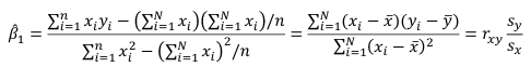
The line of best fit is the line which minimized the least squares (LS) estimate:
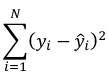
The sum of predicted minus observed values squared. For regressions with only one independent variable, X, this yields to the following equation:
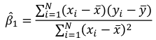
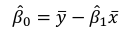
We can take the derivative with respect to each beta and set equal to 0 to end up with the following 2 equations:
Even after we find our best fit line, we cannot predict values that were outside of our sample range.
Estimated Variances of Estimates
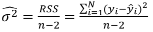
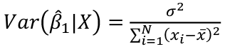
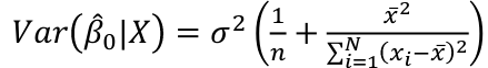
The square root of estimated variance is Standard Error (SE).
In R, the lm() function can be used to determine the simple linear regression:
res <- lm(var_y ~ var_x, data=mydata)
Sum of Squares
Model SS - SS of the differences between y predicted by the model and the overall average. (y_hat - y_bar)^2
Error SS - SS of the differences between y observed and the y predicted by the model. (yi - y_hat)^2
Total SS - SS of the differences between y observed by the model and the overall average. (yi - y_bar)^2
The better the model fits the larger the model SS and the smaller the Error SS.
F Values
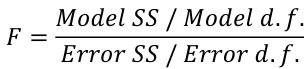
The numerator df is for the model and the denominator df is for error. In a situation with one 1 X variable, the F-test is equivalent to the t-test for the null hypothesis that β1 =0.
Also notice that in the case of one predictor, F is the square of t.
Module 14: Topics in Linear Regression
Assumption in Linear Regression:
- Independence between observations
- Linearity between X and Y
- Homoscedasticity - the variance of Y is the same for any value of X
- Normally distributed Y for any fixed value of X
Also, the model is also only generalizable to the population within the range of observed values of X.
Independence
The way we collect data or which data we collect determines independence. Examples of violated independence:
- Data comes from individuals that are related closely
- Multiple observations were collected over time for the same subject
Linearity
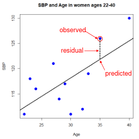
In order to test linearity, we would expect a graph of the residuals to be randomly scattered around the horizontal line. If there is a pattern to the residuals, the trend cannot be assumed to be linear.
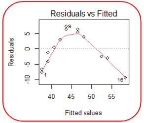
The above residual plot shows a clear trend, thus the linear assumption is voilated.
Homoscedasticity
When talking about homoscedasticity, we require variance of error terms to be similar across independent variables. To assess homoscedasticity we can look at a scatterplot of y vs. x to determine if the spread in y is the same for each value of x.
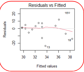
Here we observe the spread of Y increasing as X increasing, thus the homoscedasticity assumption is not met.
Normality
Finally for the normality of data we can examining the histogram of residuals and the QQ plot of residuals. If the data is normally distributed, the points will lie on the line.
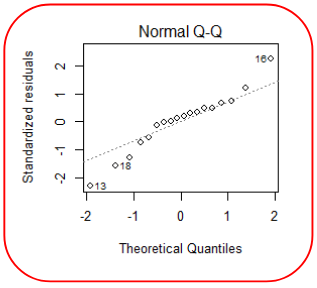
Above is a example were the QQ of the residuals indicates a violation of normality.
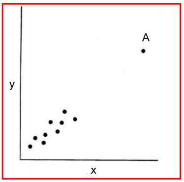
Problem Points
Problem points can be categorized as outliers, leverage points, or influential points. A point can be any or all 3.
- Outliers are defines one or more observations that has a large residual. In other words the observed value for the point is much different that that predicted by the model.
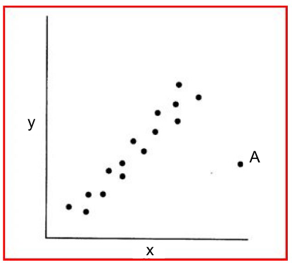
- Leverage Points are observations which have a value of x that is far away from the mean of x.
- Influential Observations is an observation that changes the slope of the line. One method to find these points is comparing the fit of the model with and without each observation.
The point A above is a leverage point, but not an outlier or an influential observation.
Here point A is an outlier and an influential observation, but not really a leverage point.
What if the assumptions are not met?
- If linearity is not met, you should consider other models (e.g. quadratic or logistic)
- If normality is not met:
- For correlation analysis we can use Spearman correlation instead of Pearson correlation
- For regression analysis, we can investigate transformations such as log or square root
Spearman Correlation
For use when data is not normally distributed. Sort the data from smallest to largest and create ranks for both X and Y, then calculate the usual correlation on the ranked values.